Purpose
Compile weather records near the Rocky Mountain Biological Laboratory in Gothic, CO and analyze long-term trends in precipitation and temperature.
library(tidyverse)
library(lubridate)
library(viridis)
library(RColorBrewer)
library(GGally)
library(ggpmisc)
library(knitr)
library(kableExtra)
knitr::opts_chunk$set(comment="", cache=T, warning = F, message = F, fig.path = "images_weather/")

maxfield_coords <- data.frame(id = "maxfield", name="MaxfieldMdw", latitude = 38.9495, longitude = -106.9908)
Datasets
WRCC
Weather data from 7 RMBL stations
- Provided by the Western Regional Climate Center, the Desert Research Institute, and the Rocky Mountain Biological Laboratory
- Raw data in metric units (cleaned “FPA” data unavailable) - lots of cleanup needed, no interspersed missing values, so may not have been quality checked at all.
- Downloaded as xls that is actually a tsv, and added quotes around each text cell, and gzipped
- Columns renamed according to metadata
- Flags on each column indicate 0 = raw data, (M)issing data, (E)stimated data, (N)on-measuring time interval
- Data for billy’s station runs 2009 - present (valid precip data starts 2015-07-01, temperature starts 2015-10-01), other stations run 2009 - 2016 and lack precip but have soil moisture
- Data are provided at 10-min intervals, so took the mean (or sum for precip) to aggregate hourly and then daily results
- Then removed some precipitation entries much greater than 50 mm/day that were interspersed with valid data
- Daily summary RData file
wrcc_metadata_noflags <- read_tsv("data/WRCC/weather_wrcc_metadata.tsv") %>% mutate(index = row_number(), flag=F)
wrcc_metadata <- bind_rows(wrcc_metadata_noflags, wrcc_metadata_noflags %>% select(name_metric, col_type, index) %>%
                             filter(! name_metric %in% c("date","time")) %>%
  mutate(name_metric=paste0("flag_",name_metric), col_type="f",flag=T)) %>% arrange(index) %>% fill(id)

#the chunk below loads the WRCC data (slow)
load("data/WRCC/daily_WRCC.rda")
get_WRCC_id <- function(filename) toupper(str_match(filename, "wrcc_([a-z]+)")[,2])
tenmin_WRCC <- list.files("data/WRCC/", ".tsv.gz", full.names=T) %>% set_names(get_WRCC_id(.)) %>%
map_dfr( ~ read_tsv(.x, skip = 4, na=c("","M"), col_types=paste0(filter(wrcc_metadata, id==get_WRCC_id(.x))$col_type, collapse=""),
col_names=filter(wrcc_metadata, id==get_WRCC_id(.x))$name_metric), .id="id")
#this comment says to "take the mean of the precip rate per hour that is reported every 10 min", but the code sums it and that matches well on the monthly scale with other stations
hourly_WRCC <- tenmin_WRCC %>% mutate(hour=hour(time)) %>% group_by(id, date, hour) %>%
summarize(precip_mm = sum(precip_mm), across(where(is.numeric), mean))
get_daily_WRCC <- function(grouped_hourly_data) {
daily <- grouped_hourly_data %>% group_by(id, .add=T) %>%
summarize(precip_mm = sum(precip_mm), #sum the hourly precip rates over each 24 hrs
max_av_temp_air_C = max(av_temp_air_C), min_av_temp_air_C = min(av_temp_air_C),
across(where(is.numeric), mean)) %>%
mutate(year=factor(year(date)), julian=yday(date),
precip_mm = ifelse(precip_mm>50 | precip_mm < 0, NA, precip_mm)) #cut nonsense precip values
}
daily_WRCC <- hourly_WRCC %>% group_by(date) %>% get_daily_WRCC()
daily_WRCC_7am <- hourly_WRCC %>% filter(id %in% c("CORBIL", "CORKET")) %>%
group_by(date = case_when(hour < 7 ~ date - days(1), hour >= 7 ~ date)) %>% get_daily_WRCC() %>%
select(id, date, year, julian, precip_mm)
save(daily_WRCC, daily_WRCC_7am, file="data/WRCC/daily_WRCC.rda")ESS-DIVE
Weather data from the Gold Link Wunderground station in Mt. Crested Butte
- Data are QAQC’d, gap-filled, and summarized hourly or daily.
- Metadata and abstract
- “This dataset is a gap-filled meteorological dataset (years 2011-2020) that includes modeled potential evapotranspiration from a station near the pumphouse on the East River (KCOMTCRE2 WeatherUnderground) near the top of the ridge at the Pumphouse PLM wells. These datasets are useful as model inputs. The KOMTCRE2 station is located on Mt. Crested Butte in Colorado. The purpose of this dataset is to use as input to hydrological and flow-reactive transport models as meteorological forcing. One attached file includes metadata files with definitions for all variables and units. Subsequent files include the same time series dataset, but aggregated and gap-filled at different time-stamp intervals. These include 5 minute time-series, 15 minute time-series, 30 minute time-series, 1 hour time-series, daily time-series, and hourly and daily modeled evapotranspiration.”
- Michelle Newcomer and David Brian Rogers. 2020. Gap-filled meteorological data (2011-2020) and modeled potential evapotranspiration data from the KCOMTCRE2 WeatherUnderground weather station, from the East River Watershed, Colorado. ESS-DIVE: Deep Insight for Earth Science Data. doi:10.15485/1734790, version: ess-dive-ce2fd798f9d81f5-20201210T030125380.
- The plot compares the daily precip calculatedd from summing the hourly precipitation rates (in mm/min), or taking the maximum daily accumulated precip. These two numbers should be the same but sometimes differ at midnight (PrecipAccum is sometimes nonzero at midnight), and sometimes when the PrecipRate does not bump up the PrecipAccum. Discrepancy might an artifact of the QA/QC applied by the authors.
hourly_KCOMTCRE2 <- read_csv("data/Wunderground/2011_2020_KComCret_60min_Measured_QAQC.csv", guess_max = 3000)
daily_KCOMTCRE2 <- read_csv("data/Wunderground/2011_2020_KComCret_1day_ETModeled.csv")

daily_KCOMTCRE2_7am <- hourly_KCOMTCRE2 %>%
  group_by(date = case_when(hr <  7 ~ date - days(1), hr >= 7 ~ date)) %>%
  summarize(Precip = sum(PrecipRate)*60) #units are mm/min

daily_KCOMTCRE2_raw <- hourly_KCOMTCRE2 %>% group_by(date) %>%
  summarize(Sum_PrecipRate = sum(PrecipRate)*60, Max_PrecipAccum = max(PrecipAccum))
ggplot(daily_KCOMTCRE2_raw) + geom_point(aes(x=Max_PrecipAccum, y=Sum_PrecipRate)) + coord_cartesian(ylim=c(0,50))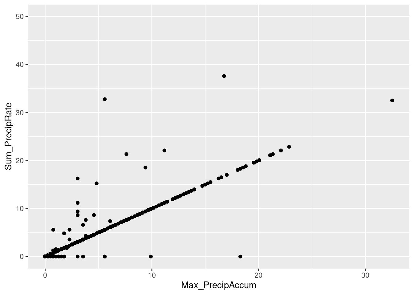
#hourly_KCOMTCRE2 %>% filter(date %in% (daily_KCOMTCRE2_raw %>% filter(abs(Max_PrecipAccum - Sum_PrecipRate > 0.01)) %>% #pull(date))) %>% ViewEPA CASTNET
Weather data from the RMBL Research Meadow
- EPA CASTNET program, station ID GTH161
- Also collects air quality data - ozone and air filters - not yet included here
- Starts in 1989 but precipitation data is missing after 2011-12-31 - suspiciously at the end of the year
- The CASTNET 2015 Factsheet says “In 2010, meteorological measurements were discontinued at most EPA-sponsored CASTNET sites due to changing priorities, which evolved based on input from policymakers and the research community. As a result, EPA developed a method to substitute historical average deposition velocities for missing MLM simulations (Bowker et al., 2011).” This is echoed in the 2010 and 2011 annual reports.
- Temperature and air quality records continue to present
- Metadata
- Provided hourly, so summarized daily, either propagating missing values or ignoring them (see code)
- The plot and table show the number of missing hourly values per day
hourly_GTH161 <- read_csv("data/EPA_CASTNET/CASTNET_GTH161_Meteorological_Hourly.csv.gz",
                          col_types=cols(DATE_TIME=col_datetime("%m/%d/%Y %H:%M:%S"), QA_CODE=col_character()))

# Tally and plot missing hourly values
hourly_GTH161_missing <- hourly_GTH161 %>% filter(DATE_TIME < ymd("2012-01-01")) %>%
  group_by(date=date(DATE_TIME)) %>% summarize(missing_precip_hrs = sum(is.na(PRECIPITATION)))
ggplot(hourly_GTH161_missing, aes(x=date, y=missing_precip_hrs)) + geom_point() +
  geom_text(data = hourly_GTH161_missing %>% count(missing_precip_hrs), aes(x=ymd("1988-01-01"), label=n))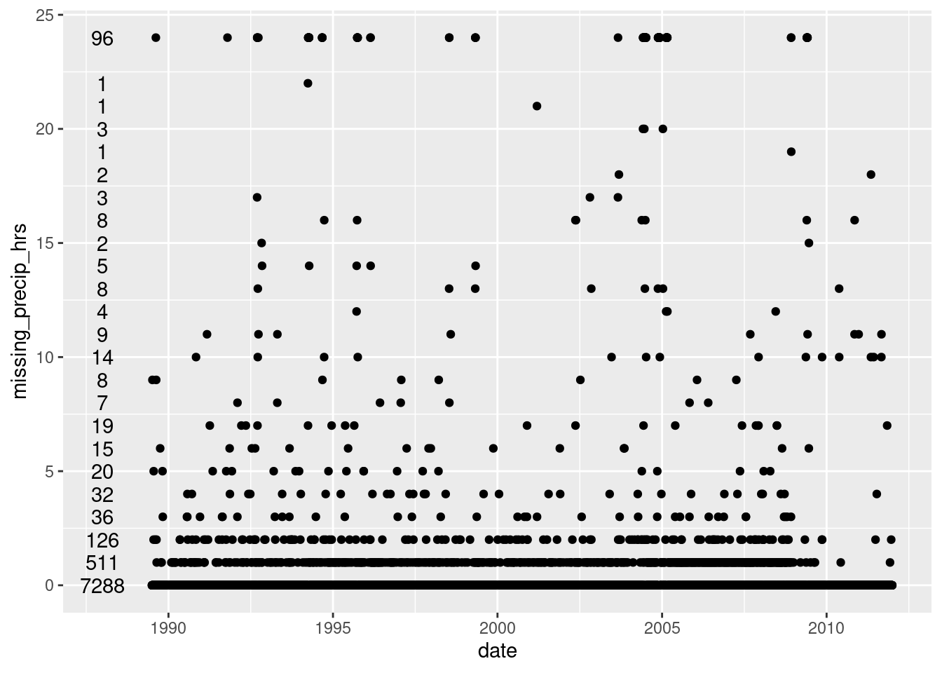
# daily_GTH161 is used for daily_all, but
# this keeps precip sums when there is missing hourly values
# an entire day missing gets precip = 0 and temperature = NaN
daily_GTH161 <- hourly_GTH161 %>% mutate(date = date(DATE_TIME)) %>% filter(year(date) < 2012) %>% group_by(date) %>%
  summarize(TEMPERATURE=mean(TEMPERATURE, na.rm=T), PRECIPITATION = sum(PRECIPITATION, na.rm=T))

# daily_GTH161_NA propagates any missing hourly values up to the day.
daily_GTH161_NA <- hourly_GTH161 %>% arrange(DATE_TIME) %>% group_by(date = date(DATE_TIME)) %>%
    summarize(tavg_C=mean(TEMPERATURE), tmax_C=max(TEMPERATURE), tmin_C=min(TEMPERATURE),
              prcp_mm = sum(PRECIPITATION), across(where(is.numeric), mean))
# Could be customized to accept a few missing hours with maxNA:
#summarizeNA <- function(x, fun, maxNA = 0) {
#  ifelse(sum(is.na(x)) <= maxNA, fun(x, na.rm=T), NA)
#}

# daily_GTH161_NA_7am counts precipitation occurring BEFORE 7 am as the previous day, to
# line up with CoCoRaHs datasets that I shifted one day back
daily_GTH161_NA_7am <- hourly_GTH161 %>% arrange(DATE_TIME) %>%
  group_by(date = case_when(hour(DATE_TIME) <  7 ~ date(DATE_TIME) - days(1),
                            hour(DATE_TIME) >= 7 ~ date(DATE_TIME))) %>%
    summarize(tavg_C=mean(TEMPERATURE), tmax_C=max(TEMPERATURE), tmin_C=min(TEMPERATURE),
              prcp_mm = sum(PRECIPITATION), across(where(is.numeric), mean))
NOAA
Weather data from 7 stations near RMBL sourced from NOAA’s GHCN Daily dataset.
- All stations within 10 km of Maxfield Meadow near Gothic
- Daily summaries quality checked by GHCN
- Includes long records from Crested Butte (1909-present), Schofield Pass (1985-present), Butte (1980-present)
- The Crested Butte station precip is collected at 9:00 am, but the collection time is unknown for Schofield Pass and Butte, which are probably automated (midnight-midnight)
- Stations beginning with US1COGN (Colorado-Gunnison County) are community CoCoRaHS stations, including billy barr’s station in Gothic. Unlike some the other datasets, the reported precipitation is from 7 am the previous day to 7 am that day, according to CoCoRaHS. For some stations, it ranges from 6:30-8:00 am.
- To handle this discrepancy coarsely, the date is set to the day before on CoCoRaHS stations and NOAA Crested Butte, since most hours of precip are from day prior, and most summer precipitation is in the afternoon.
- Then in compared hourly datasets (EPA, WRCC, ESSDIVE), the date is set to the day prior for precip collected before 7 am.
library(rnoaa)
station_data <- ghcnd_stations()# long download unless cached
NOAA_stations <- meteo_nearby_stations(lat_lon_df = maxfield_coords, station_data = station_data,
                      var = c("PRCP", "TAVG"), radius = 10)$maxfield %>% #stations within 10 km radius of Maxfield
    left_join(station_data %>% filter(element=="PRCP")) %>%
  mutate(CoCoRaHS = str_sub(id,1,3) == "US1")
remove(station_data)
NOAA_stations_name <- with(NOAA_stations, set_names(name, id))
NOAA_stations_morning <- NOAA_stations %>% filter(CoCoRaHS) %>% pull(id) %>% c("USC00051959") #Crested Butte is collected in the morning too, at 9am

daily_NOAA <- meteo_pull_monitors(NOAA_stations$id, keep_flags = T) %>%
  mutate(across(contains("flag"), as.factor)) %>% #All units are in tenths of mm, converted to mm here.
  mutate(across(c("prcp","snow","snwd","wesd","wesf"), ~ as.integer(.x)/10, .names="{.col}_mm"), .keep="unused") %>%
  mutate(across(c("tmin","tavg","tmax"), ~ as.integer(.x)/10, .names="{.col}_C"), .keep="unused") %>%
  mutate(date = case_when(id %in% NOAA_stations_morning ~ date - days(1), TRUE ~ date)) %>% # CoCoRaHS stations are recorded the next day at 7 am (and CB at 9 am), so set them back a day
  mutate(prcp_mm = ifelse(id=="USC00051959" & date %in% c(ymd("2000-08-03"),ymd("2018-07-28")), NA, prcp_mm)) #cut 2 extreme precip values at CB station not recorded by other stations
CoCoRaHS
Community precipitation monitoring stations using manual gauges emptied in the morning (around 7 am local).
- The NOAA dataset includes a few of these stations
- Daily reports exported from directly from CoCoRaHS for Gunnison County, CO since 2000
- Plots of data coverage and observation times, table of currently active stations
- See complete Gunnison County station list
daily_CoCoRaHS <- read_csv("data/NOAA_GHCN/CoCoRaHS_DailyPrecipReports_CO_GN.csv", guess_max=1e4) %>%
  mutate(across(TotalPrecipAmt:TotalSnowSWE, ~25.4*as.numeric(.x)),# T(race) to NA, convert inches to mm
         across(starts_with("Station"), factor))

ggplot(daily_CoCoRaHS, aes(x=ObservationDate, y=StationName, fill=TotalPrecipAmt)) + geom_tile()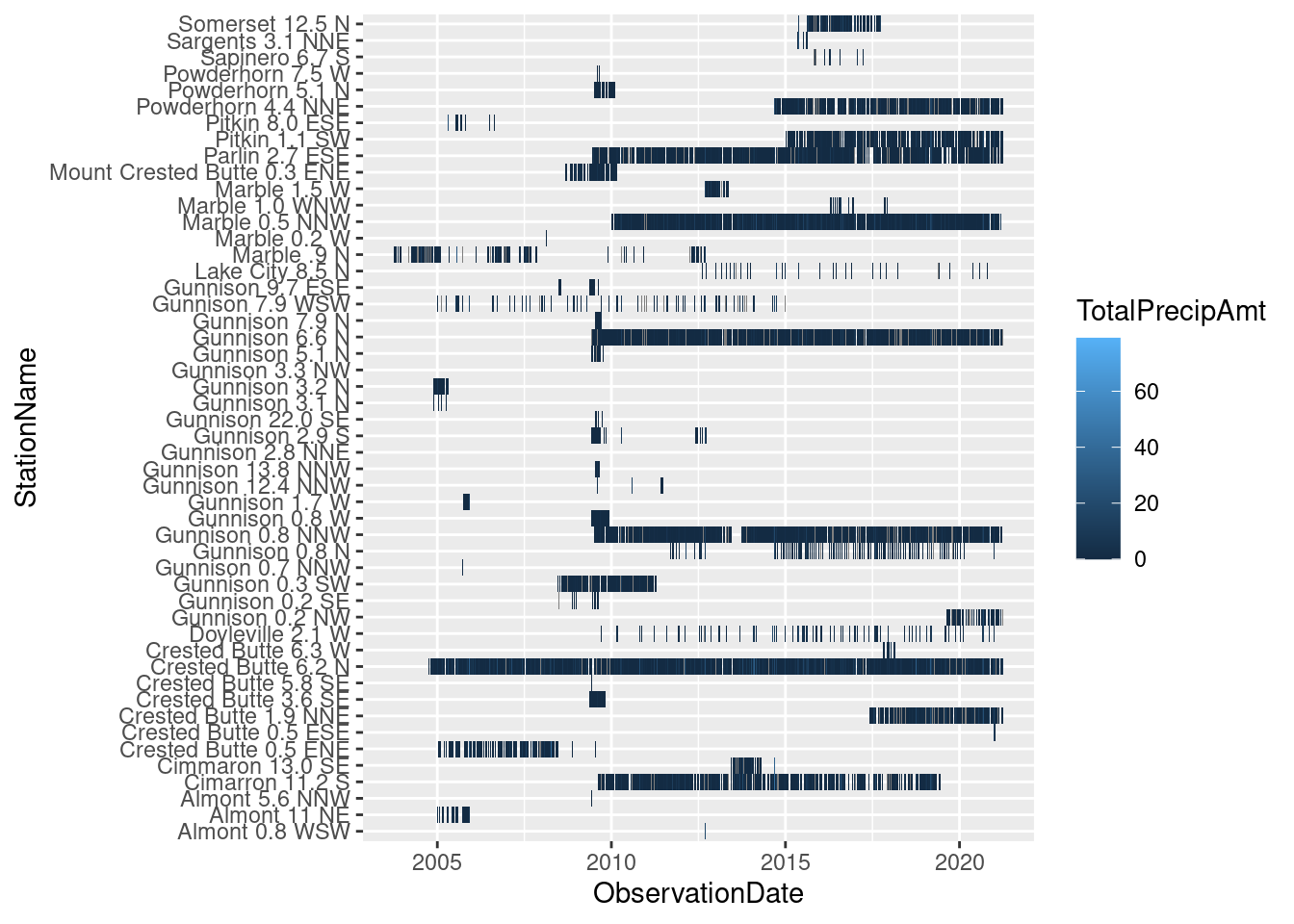
ggplot(daily_CoCoRaHS, aes(x=ObservationTime, y=StationName)) + geom_point(shape=1, alpha=0.2)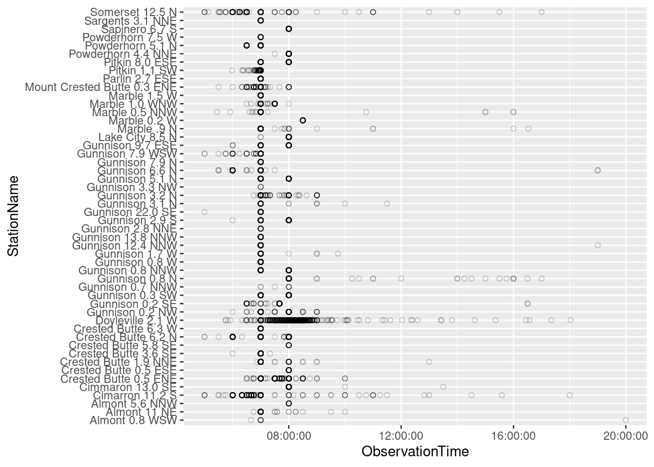
CoCoRaHS_stations <- daily_CoCoRaHS %>% group_by(StationName, StationNumber) %>%
  summarize(across(c(Latitude, Longitude), unique), medianObservationTime=median(ObservationTime)) %>%
  left_join(read_tsv("data/NOAA_GHCN/CoCoRaHS_Stations_CO_GN.tsv"))

CoCoRaHS_stations %>% mutate(StationNumber = cell_spec(StationNumber, "html", link = Link), .keep="unused") %>%
  select(-c(Type, State, County, OldStationNumber)) %>% filter(Active=="Yes") %>%
kable("html", escape = FALSE) %>% kable_styling(bootstrap_options = c("hover", "condensed")) | StationName | StationNumber | Latitude | Longitude | medianObservationTime | Active |
|---|---|---|---|---|---|
| Cimarron 11.2 S | CO-GN-47 | 38.28847 | -107.5550 | 07:00:00 | Yes |
| Crested Butte 0.5 ESE | CO-GN-70 | 38.86734 | -106.9741 | 08:00:00 | Yes |
| Crested Butte 1.9 NNE | CO-GN-66 | 38.89471 | -106.9685 | 07:00:00 | Yes |
| Crested Butte 6.2 N | CO-GN-18 | 38.96030 | -106.9908 | 07:00:00 | Yes |
| Crested Butte 6.3 W | CO-GN-67 | 38.87571 | -107.0998 | 07:00:00 | Yes |
| Doyleville 2.1 W | CO-GN-49 | 38.42486 | -106.6192 | 08:00:00 | Yes |
| Gunnison 0.2 NW | CO-GN-68 | 38.54689 | -106.9296 | 07:00:00 | Yes |
| Gunnison 0.8 N | CO-GN-52 | 38.55570 | -106.9286 | 08:00:00 | Yes |
| Gunnison 0.8 NNW | CO-GN-41 | 38.54020 | -106.9238 | 08:00:00 | Yes |
| Gunnison 2.8 NNE | CO-GN-71 | 38.58036 | -106.9031 | 07:00:00 | Yes |
| Gunnison 6.6 N | CO-GN-40 | 38.63912 | -106.9408 | 07:00:00 | Yes |
| Lake City 8.5 N | CO-GN-54 | 38.15131 | -107.2982 | 08:00:00 | Yes |
| Marble 0.5 NNW | CO-GN-50 | 39.07911 | -107.1906 | 07:00:00 | Yes |
| Parlin 2.7 ESE | CO-GN-39 | 38.48433 | -106.6742 | 07:00:00 | Yes |
| Pitkin 1.1 SW | CO-GN-59 | 38.59850 | -106.5313 | 07:00:00 | Yes |
| Powderhorn 4.4 NNE | CO-GN-58 | 38.34010 | -107.0943 | 08:00:00 | Yes |
NCEI
Weather data from the Global Surface Summary of the Day (GSOD)
- From NOAA’s National Centers for Environmental Information (NCEI)
- Not currently imported - only get Gunnison/Crested Butte and Aspen airports
- List of stations
library(GSODR)
gsodr.inventory <- get_inventory() %>% #long download
  filter(STNID %in% nearest_stations(38.9495, -106.9908,50))
gothicwx
billy barr’s snow records in Gothic, CO
groundcover <- read_tsv("./data/gothicwx/groundcover.tsv") %>%
  mutate(across(starts_with("first"), list(day=yday)), year=year(first_0_cm))

groundcover_2023 <- tibble(first_snow=ymd("2022-10-23"), first_0_cm=ymd("2023-05-01"))
#TODO fill in actual value for first_0_cm in 2023

get_seasons <- function(dates) {
  factor(c("smmr","wntr"))[ifelse(year(dates) < min(groundcover$year), NA,
         1+dates %in% do.call(c,
                             map2(bind_rows(groundcover, groundcover_2023)$first_snow,
                                  bind_rows(groundcover, groundcover_2023)$first_0_cm,
                                  ~ seq(date(.x), date(.y), by="day"))))]
}
Combine datasets
Combine selected daily weather station data in long or wide format.
#Combine a few of the closer weather station precipitation datasets and snowmelt in wide format
daily_all <-
  daily_NOAA %>% filter(id == "US1COGN0018") %>%
  full_join(daily_GTH161) %>% full_join(daily_KCOMTCRE2) %>%
  full_join(daily_WRCC %>% filter(id=="CORBIL"), by="date") %>%
  rename(EPA_RsrchMdw=PRECIPITATION, ESSDIVE_GoldLink=Precip, WRCC_billy=precip_mm, NOAA_billy=prcp_mm) %>%
  mutate(yr = year(date), mo = month(date, label=F),
         ground_covered = get_seasons(date)) %>% filter(year(date) < 2023)

#Combine all the weather stations daily precip and temperature statistics in long format
daily_long <- bind_rows(
  GTH161 = daily_GTH161_NA %>% select(date, tavg_C, tmax_C, tmin_C, prcp_mm),
  KCOMTCRE2 = daily_KCOMTCRE2 %>% select(date, tavg_C = Tmean, tmax_C = Tmax, tmin_C = Tmin, prcp_mm = Precip),
  .id="id") %>%
  bind_rows(daily_WRCC %>% select(id, date, tavg_C = av_temp_air_C,
                                  tmax_C = max_av_temp_air_C, tmin_C = min_av_temp_air_C,
                                  prcp_mm = precip_mm)) %>%
  bind_rows(daily_NOAA %>% select(id, date, tavg_C, tmax_C, tmin_C, prcp_mm)) %>% mutate(id=factor(id))%>% filter(year(date) < 2023)

# The datasets summarized to line up with the morning collections
daily_long_7am <- bind_rows(
  GTH161 = daily_GTH161_NA_7am %>% select(date, prcp_mm),
  KCOMTCRE2 = daily_KCOMTCRE2_7am %>% select(date, prcp_mm = Precip), .id="id") %>%
  bind_rows(daily_WRCC_7am %>% select(id, date, prcp_mm = precip_mm)) %>%
  bind_rows(daily_NOAA %>% select(id, date, prcp_mm)) %>% # morning stations shifted back a day
  mutate(ground_covered = get_seasons(date)) %>% filter(year(date) < 2023)

daily_all_7am <- daily_long_7am %>%
  pivot_wider(names_from="id", values_from="prcp_mm") %>% arrange(date)
Stations
Metadata
List the weather station metadata
- Links point to the data sources
- Distance is from Maxfield Meadow
- Years show the range of the precipitation record (NA if no precipitation data)
all_stations <- bind_rows(
  NOAA_stations %>% mutate(source="NOAA", url=paste0("https://www.ncdc.noaa.gov/cdo-web/datasets/GHCND/stations/GHCND:",id,"/detail")),
  read_tsv("data/stations.tsv") %>%
  rnoaa::meteo_process_geographic_data(lat = maxfield_coords$latitude, long = maxfield_coords$long) %>%
    mutate(element="PRCP")) %>%
  mutate(source_name = paste(source, name, sep="_"),
         short_name = str_replace(name, "CRESTED BUTTE","CB"),
         color = c(brewer.pal(8, "Set1")[1:6],"grey80", brewer.pal(8, "Set1")[7:8],"black", brewer.pal(9, "Set1")[9], brewer.pal(6, "Dark2"))) %>%
  rows_patch(daily_long %>% drop_na(prcp_mm)  %>% group_by(id) %>% summarize(first_year=min(year(date)), last_year=max(year(date))))
stations_pal <- with(all_stations, set_names(color, short_name))
stations_name <- with(all_stations, set_names(short_name, id))
stations_source_name <- with(all_stations, set_names(source_name, id))

all_stations %>% select(-c(state, gsn_flag, wmo_id, source_name, short_name, color)) %>% relocate(source) %>%
  write_tsv("data/all_stations.tsv") %>%
  mutate(id = cell_spec(id, "html", link = url), .keep="unused") %>%
kable("html", escape = FALSE) %>% kable_styling(bootstrap_options = c("hover", "condensed")) | source | id | name | latitude | longitude | distance | elevation | element | first_year | last_year | CoCoRaHS |
|---|---|---|---|---|---|---|---|---|---|---|
| NOAA | US1COGN0018 | CRESTED BUTTE 6.2 N | 38.96030 | -106.9908 | 1.2009052 | 2927.9 | PRCP | 2004 | 2023 | TRUE |
| NOAA | US1COGN0030 | MOUNT CRESTED BUTTE 0.3 ENE | 38.91030 | -106.9623 | 5.0076927 | 2941.0 | PRCP | 2008 | 2010 | TRUE |
| NOAA | US1COGN0066 | CRESTED BUTTE 1.9 NNE | 38.89470 | -106.9685 | 6.3915733 | 2822.4 | PRCP | 2017 | 2023 | TRUE |
| NOAA | USS0006L11S | Butte | 38.89000 | -106.9500 | 7.4987757 | 3096.8 | PRCP | 1980 | 2023 | FALSE |
| NOAA | USC00051959 | CRESTED BUTTE | 38.87390 | -106.9772 | 8.4882935 | 2702.7 | PRCP | 1909 | 2023 | FALSE |
| NOAA | US1COGN0020 | CRESTED BUTTE 0.5 ENE | 38.87220 | -106.9780 | 8.6664240 | 2706.0 | PRCP | 2004 | 2011 | TRUE |
| NOAA | US1COGN0070 | CRESTED BUTTE 0.5 ESE | 38.86730 | -106.9741 | 9.2537385 | 2700.8 | PRCP | 2018 | 2023 | TRUE |
| NOAA | USS0007K11S | Schofield Pass | 39.02000 | -107.0500 | 9.3614039 | 3261.4 | PRCP | 1985 | 2022 | FALSE |
| EPA | GTH161 | RsrchMdw | 38.95627 | -106.9859 | 0.8651189 | 2915.0 | PRCP | 1989 | 2011 | NA |
| EPA_NOAA | EPA_NOAA_filled | RsrchMdw_filled | 38.95627 | -106.9859 | 0.8651189 | 2915.0 | PRCP | NA | NA | NA |
| WRCC | CORBIL | billy | 38.96300 | -106.9930 | 1.5131369 | 2917.0 | PRCP | 2015 | 2021 | NA |
| WRCC | CORJUD | JuddFalls | 38.96400 | -106.9840 | 1.7161922 | 3004.0 | PRCP | NA | NA | NA |
| WRCC | CORKET | KettlePonds | 38.94200 | -106.9730 | 1.7507490 | 2860.0 | PRCP | 2015 | 2016 | NA |
| WRCC | CORSNO | Snodgrass | 38.93300 | -106.9860 | 1.8810956 | 3396.0 | PRCP | NA | NA | NA |
| ESSDIVE | KCOMTCRE2 | GoldLink | 38.91500 | -106.9590 | 4.7204356 | 2926.0 | PRCP | 2011 | 2020 | NA |
| WRCC | CORMEX | MexicanCut | 39.02800 | -107.0640 | 10.7804142 | 3412.0 | PRCP | NA | NA | NA |
| WRCC | CORALM | Almont | 38.65500 | -106.8620 | 34.5967136 | 2469.0 | PRCP | NA | NA | NA |
Map
Map of stations, excluding Almont
library(OpenStreetMap)
map <- openmap(c(39.05, -107.1), c(38.85, -106.9), type="opencyclemap")#, type = "stamen-terrain"
map.latlon <- openproj(map, projection = "+proj=longlat +ellps=WGS84 +datum=WGS84 +no_defs")
OpenStreetMap::autoplot.OpenStreetMap(map.latlon) +
  geom_point(data=filter(all_stations, !(id %in% c("CORALM", "EPA_NOAA_filled"))),
             aes(x=longitude, y=latitude, color=short_name), size=2) +
  theme(legend.position="bottom", axis.title=element_blank()) + labs(color="Station") +
  scale_color_manual(values=stations_pal)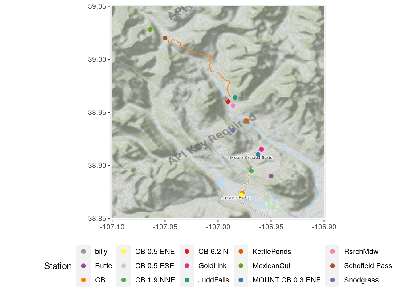
Data coverage
The range that each station was active collecting precipitation or temperature data. Note that data have not been cleaned at all yet, so there are unrealistic extreme values.
ggplot(daily_long, aes(x=date, y=id, fill=prcp_mm)) + geom_tile() +
  scale_y_discrete(labels=stations_source_name) +
  labs(y="Station",x="Year", fill="Daily precipitation (mm)") +
  theme_minimal() + theme(legend.position = "top")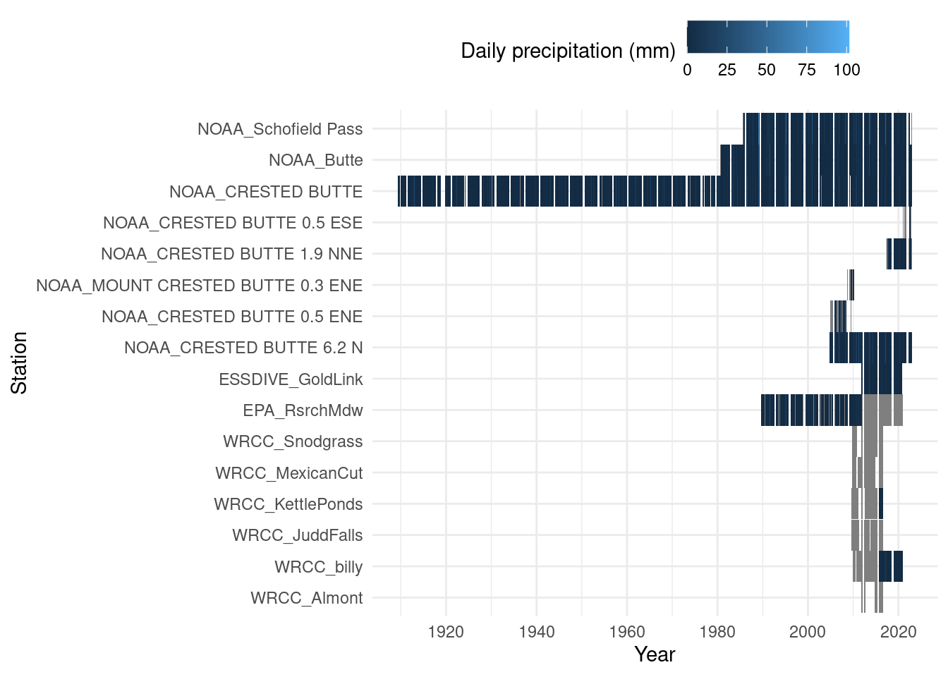
ggplot(daily_long, aes(x=date, y=id, fill=tmax_C)) + geom_tile() +
  scale_y_discrete(labels=stations_source_name) + scale_color_viridis_c(option="inferno") +
  labs(y="Station",x="Year", fill="Maximum temperature (C)") +
  theme_minimal() + theme(legend.position = "top")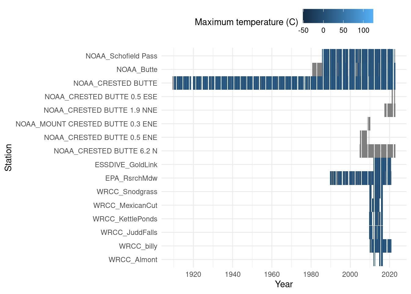
Compare daily precip
Compare summer precipitation data across stations.
- The correlation plots show how precipitation measurements are correlated on the daily scale, after shifting the stations with morning collections back a day and grouping measurements in the hourly datasets before 7 am to the previous day.
- Only summer data is shown in the correlation plot, as determined by billy’s gothicwx groundcover data.
- View the full correlation plot matrix to compare all the stations.
daily_long_7am %>% mutate(yr = year(date)) %>%
  filter(yday(date) >100, yday(date) < 240, yr %in% 2018:2020) %>%
  ggplot(aes(x=yday(date), y=prcp_mm, color=stations_name[id], shape=ground_covered)) +
  geom_point() + facet_wrap(vars(yr)) + scale_color_manual(values=stations_pal) + #ncol=1
  labs(x="Day of year", y = "Precipitation (mm)", color="Station", shape="Snow cover") +
  theme(legend.position = "top")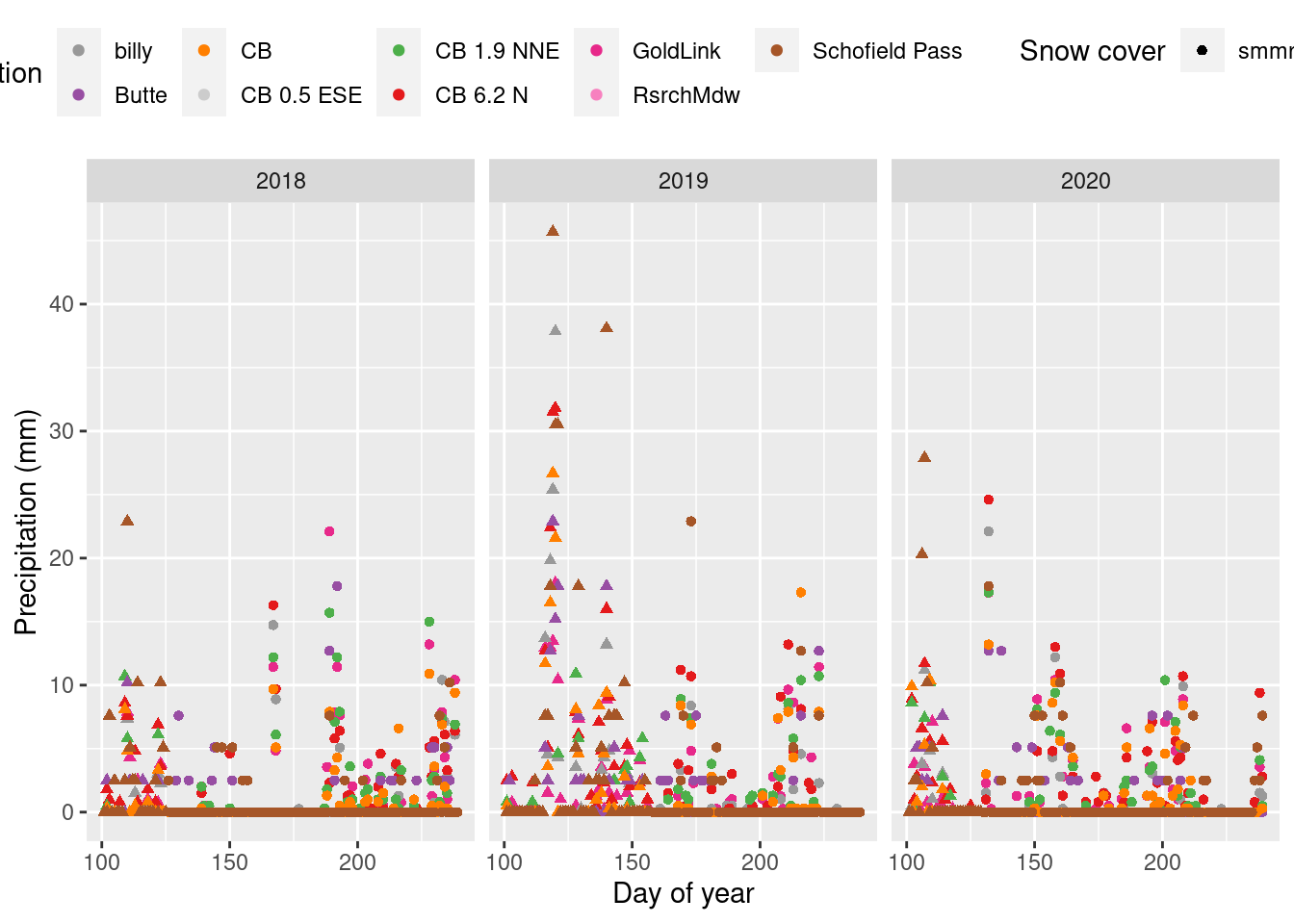
ggcorr(daily_all_7am %>% filter(ground_covered=="smmr") %>%
          select(-c(date, ground_covered)) %>% rename_with(~ stations_source_name[.x]),
       layout.exp=0.5, geom="tile", label_size=3, label=T, name="r", hjust = .9, size = 2.5)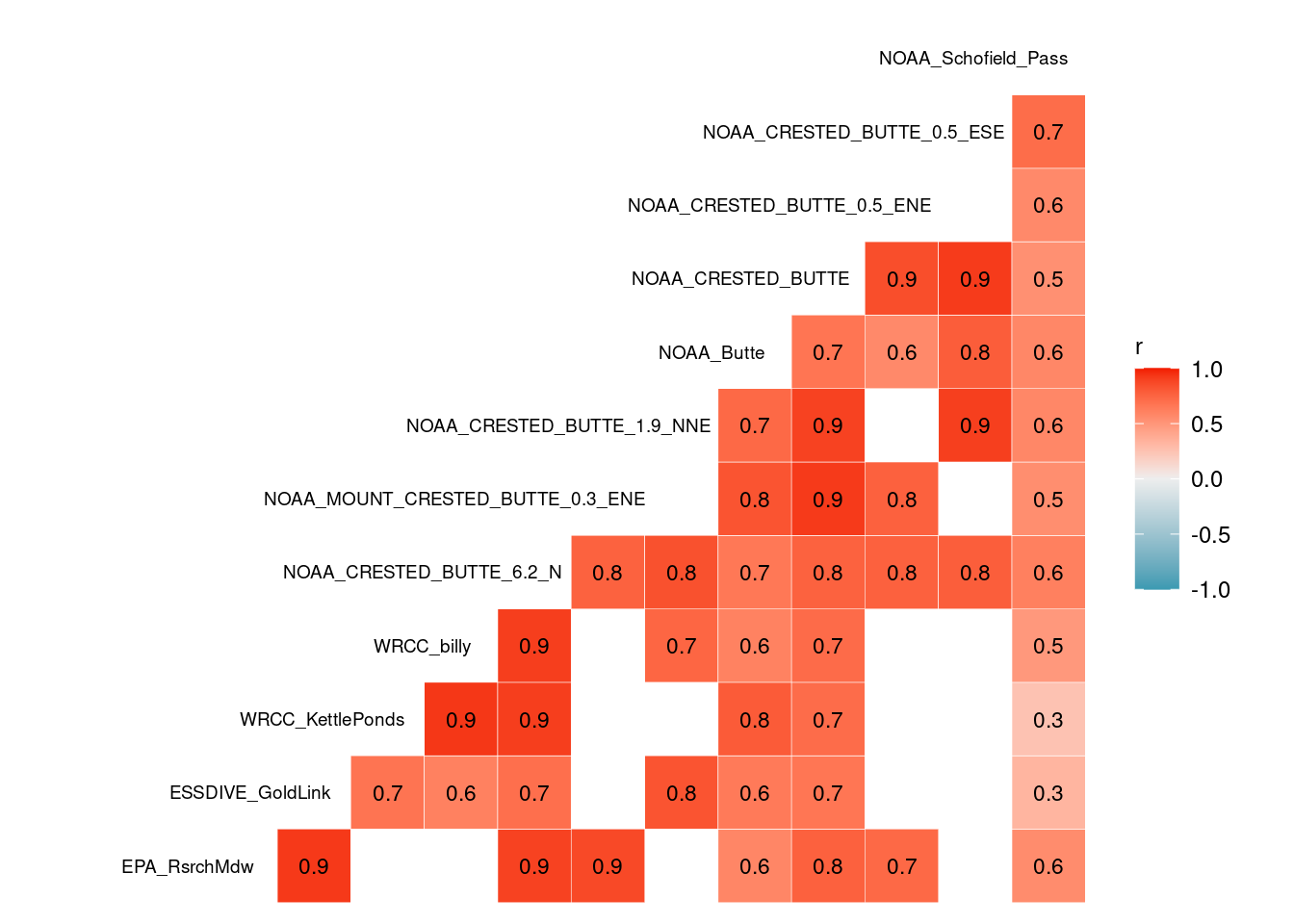
precip_max <- 50
scatter_continuous <- function (data, mapping, method="p", use="pairwise", ...) {
  corr <- cor(eval_data_col(data, mapping$x), eval_data_col(data, mapping$y), method=method, use=use)
  colFn <- colorRampPalette(c("blue", "white", "red"), interpolate ='spline')
  fill <- colFn(100)[findInterval(corr, seq(-1, 1, length=100))]
  ggally_smooth(data = data, mapping = mapping, ..., method = "loess", color="blue", se=F, span=0.3) +
    ggplot2::annotate("text", x=40, y=10, label = round(corr,2))+
        theme_classic() + theme(panel.background = element_rect(fill=fill)) +
    scale_shape_manual(values=c(1,2))+
    coord_cartesian(xlim=c(0,precip_max), ylim=c(0,precip_max)) + geom_abline(slope=1, intercept=0)+
    scale_x_continuous(breaks=seq(0,precip_max, by=precip_max/5))+
    scale_y_continuous(breaks=seq(0,precip_max, by=precip_max/5))
}
facethist_combo <- function (data, mapping, ...) {
    ggally_facethist(data = data, mapping = mapping, binwidth=precip_max/50,...) +
    coord_cartesian(xlim=c(0,precip_max)) + scale_x_continuous(breaks=seq(0,precip_max, by=precip_max/5))
}
corrplot_7am <- ggpairs(daily_all_7am %>% filter(ground_covered=="smmr") %>%
          select(-c(date, ground_covered)) %>% rename_with(~ stations_name[.x]),
        lower=list(continuous=wrap(scatter_continuous), na="blank"),
        upper=list(continuous=wrap(scatter_continuous), na="blank"))
ggsave("images_weather/corrplot_7am.pdf", corrplot_7am, device=cairo_pdf, height=10, width=12)
Fill in Research Meadow precip data
EPA precip data from the Research Meadow ends in 2011 and has some small gaps that need to be filled in to get accurate summer totals.
- For both of these methods, the EPA precipitation data (GTH161) is summed from 7 am to 7 am to match the collections at CoCoRaHs stations and NOAA Crested Butte (actually 9 am), and count hours before 7am as the previous day
Regression method - not used
- Uses a simple linear model for their period of overlap, forced through zero
- Fit separately for summer vs. winter (determined by billy’s groundcover data)
- billy’s Gothic CoCoRaHs data fills gaps from 2012-present, and small gaps from 2004-2011 (US1COGN0018, summer r = 0.90)
- Before that (1989-2004), small gaps are filled with a similar regression to the NOAA Crested Butte station (USC00051959, summer r = 0.75)
- Regressions are not a great method since they are influenced strongly by large precip events
- Give different slopes when run on daily or monthly scales
- Use the Normal Ratio Method instead (see below)
# EPA_billy_daily_model <-  lm(GTH161 ~ US1COGN0018:ground_covered + 0, data=daily_all_7am)
# EPA_CB_daily_model <-     lm(GTH161 ~ USC00051959:ground_covered + 0, data=daily_all_7am)
#
# daily_filled_7am <- daily_all_7am %>%
#   mutate(EPA_NOAA_source = ifelse(is.na(GTH161), ifelse(!is.na(US1COGN0018), "US1COGN0018",
#                                                                ifelse(!is.na(USC00051959), "USC00051959", NA)), "GTH161"),
#          EPA_NOAA_filled = ifelse(is.na(GTH161), ifelse(!is.na(US1COGN0018), predict(EPA_billy_daily_model),
#                                                         ifelse(!is.na(USC00051959), predict(EPA_CB_daily_model), NA)), GTH161))

monthly_all_7am <- daily_all_7am %>% group_by(yr = year(date), mo = month(date)) %>%
  summarize(across(-c(date, ground_covered),
                   ~ ifelse(sum(is.na(.x))>5, NA, sum(.x, na.rm=T))), .groups="drop") %>%  #tolerate 5 missing days
  arrange(yr, mo)

library(gridExtra)
grid.arrange(
  ggplot(daily_all_7am, aes(y=GTH161, x= US1COGN0018, color=ground_covered)) + coord_fixed()+
  geom_point(shape=1) + geom_smooth(span=0.3, se=F) + geom_smooth(method="lm", se=F) + geom_abline(intercept=0, slope=1) +
   stat_poly_eq(formula = y ~ x + 0, aes(label = paste(..eq.label..,"x", ..rr.label.., sep = "~~~")), parse = T) +
  labs(color="Snow cover", y=stations_source_name["GTH161"], x=stations_source_name["US1COGN0018"], title="Daily totals"),
ggplot(monthly_all_7am %>%  mutate(season=factor(c("Oct-May","Jun-Sept"))[1+mo %in% 6:9]),
       aes(y=GTH161, x= US1COGN0018, color=season)) + coord_fixed()+
  geom_point(shape=1) + geom_smooth(span=0.6, se=F) + geom_smooth(method="lm", formula= y ~ x + 0, se=F) + geom_abline(intercept=0, slope=1) +
   stat_poly_eq(formula = y ~ x + 0, aes(label = paste(..eq.label..,"x", ..rr.label.., sep = "~~~")), parse = T) +
  labs(color="Season", y=stations_source_name["GTH161"], x=stations_source_name["US1COGN0018"], title="Monthly totals"))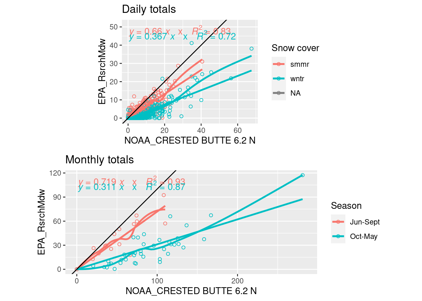
grid.arrange(
ggplot(daily_all_7am, aes(y=GTH161, x= USC00051959, color=ground_covered)) + coord_fixed()+
  geom_point(shape=1) + geom_smooth(method="lm", se=F) + geom_abline(intercept=0, slope=1) +
   stat_poly_eq(formula = y ~ x + 0, aes(label = paste(..eq.label..,"x", ..rr.label.., sep = "~~~")), parse = T) +
  labs(color="Snow cover", y=stations_source_name["GTH161"], x=stations_source_name["USC00051959"], title="Daily totals"),
ggplot(monthly_all_7am %>%  mutate(season=factor(c("Oct-May","Jun-Sept"))[1+mo %in% 6:9]),
       aes(y=GTH161, x= USC00051959, color=season)) + coord_fixed()+
  geom_point(shape=1) + geom_smooth(span=0.6, se=F) + geom_smooth(method="lm", formula= y ~ x + 0, se=F) + geom_abline(intercept=0, slope=1) +
   stat_poly_eq(formula = y ~ x + 0, aes(label = paste(..eq.label..,"x", ..rr.label.., sep = "~~~")), parse = T) +
  labs(color="Season", y=stations_source_name["GTH161"], x=stations_source_name["USC00051959"], title="Monthly totals"))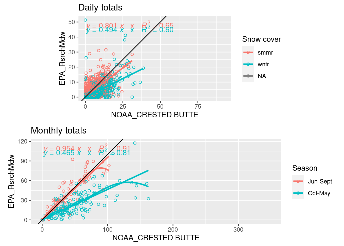
ggplot(daily_all_7am, aes(y=US1COGN0018, x= USC00051959, color=ground_covered)) + coord_fixed()+
  geom_point(shape=1) + geom_smooth(method="lm", se=F) + geom_abline(intercept=0, slope=1) +
   stat_poly_eq(formula = y ~ x + 0, aes(label = paste(..eq.label..,"x", ..rr.label.., sep = "~~~")), parse = T) +
  labs(color="Snow cover", y=stations_source_name["US1COGN0018"], x=stations_source_name["USC00051959"], title="Daily totals")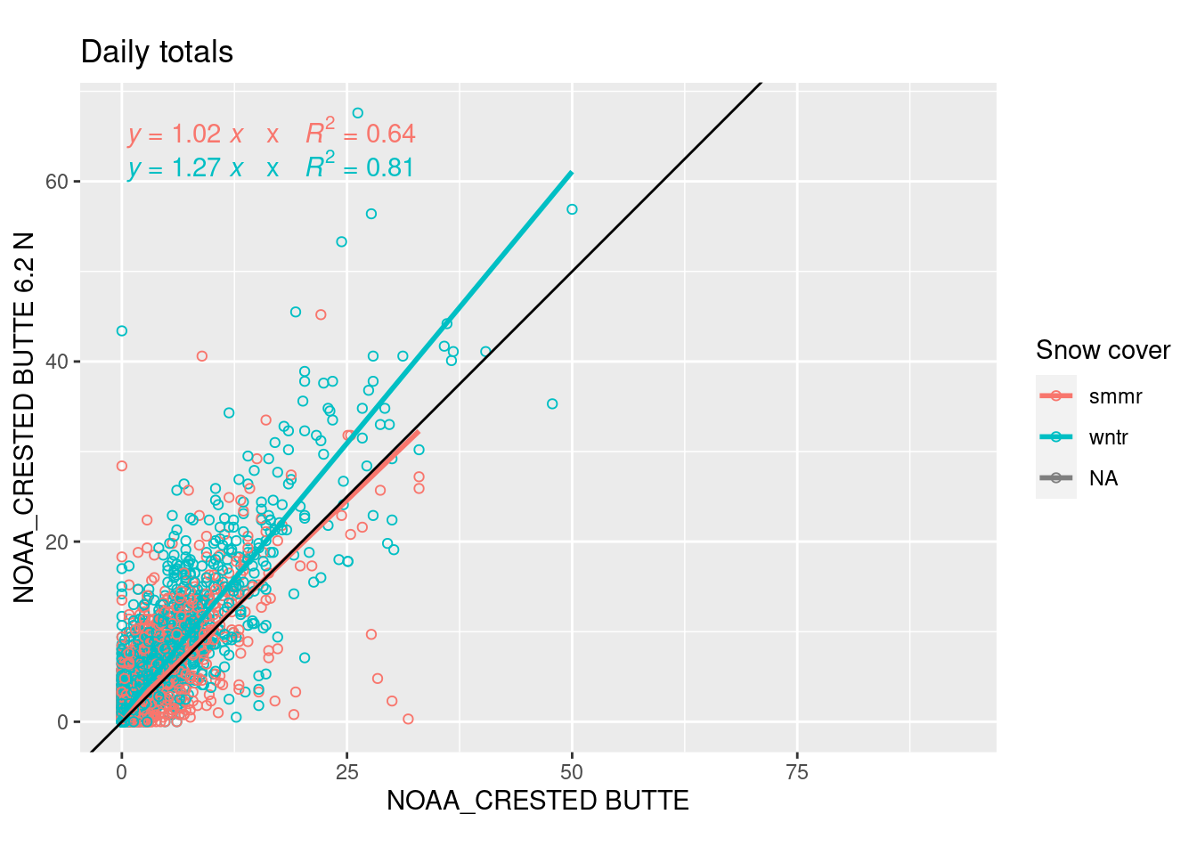
Normal ratio method
This method uses the ratio between the average annual precipitation at each station to fill in missing values.
- I adapted it to use the average of the ratios across years (since only some years overlap and the average is changing with cliamte change)
- I only consider summer precipitation, since winter precip is less easily measured and the ratios differ
- The plot compares the ratios of total summer/winter precip (determined by billy’s groundcover data) to the NOAA Crested Butte station (CB)
- The EPA vs. CB summer ratio is usually close to 1 and not that variable, so all of the missing data are filled from CB.
- Guide to some precipitation imputation methods
- In a paper comparing precipitation imputation methods, known as the “UK traditional method”
# total summer or winter precip relative to CB station
# calculated as daily average for each station across the season, dropping missing values
relative_to_CB <- daily_all_7am %>% drop_na(ground_covered) %>%
  group_by(year=year(date), ground_covered) %>% summarize(across(-c(date), ~mean(.x, na.rm=T)/mean(USC00051959, na.rm=T)))

relative_to_CB %>% pivot_longer(-c(year, ground_covered), names_to="id", values_to="prcp_rel_CB") %>% drop_na(prcp_rel_CB) %>%
  ggplot(aes(y=stations_source_name[id], x=prcp_rel_CB, color=ground_covered))+
  geom_vline(xintercept=1) + geom_boxplot() + scale_x_continuous(breaks=0:6, limits=c(0,4.1))+
  labs(x="Mean daily precipitation relative to Crested Butte", y="", color="Snow cover") + theme(legend.position = "top")
relative_to_CB %>% pivot_longer(-c(year, ground_covered), names_to="id", values_to="prcp_rel_CB") %>% drop_na(prcp_rel_CB) %>%
  #group_by(year, ground_covered) %>% summarize(prcp_rel_CB=mean(prcp_rel_CB)) %>%
  ggplot(aes(color=stations_name[id], x= year, y=prcp_rel_CB, linetype=ground_covered))+ geom_line(size=1)+
  scale_color_manual(values=stations_pal)+ ylim(c(0,4.1))+
  labs(x="Mean daily precipitation relative to Crested Butte", y="", color="Snow cover") + theme(legend.position = "top")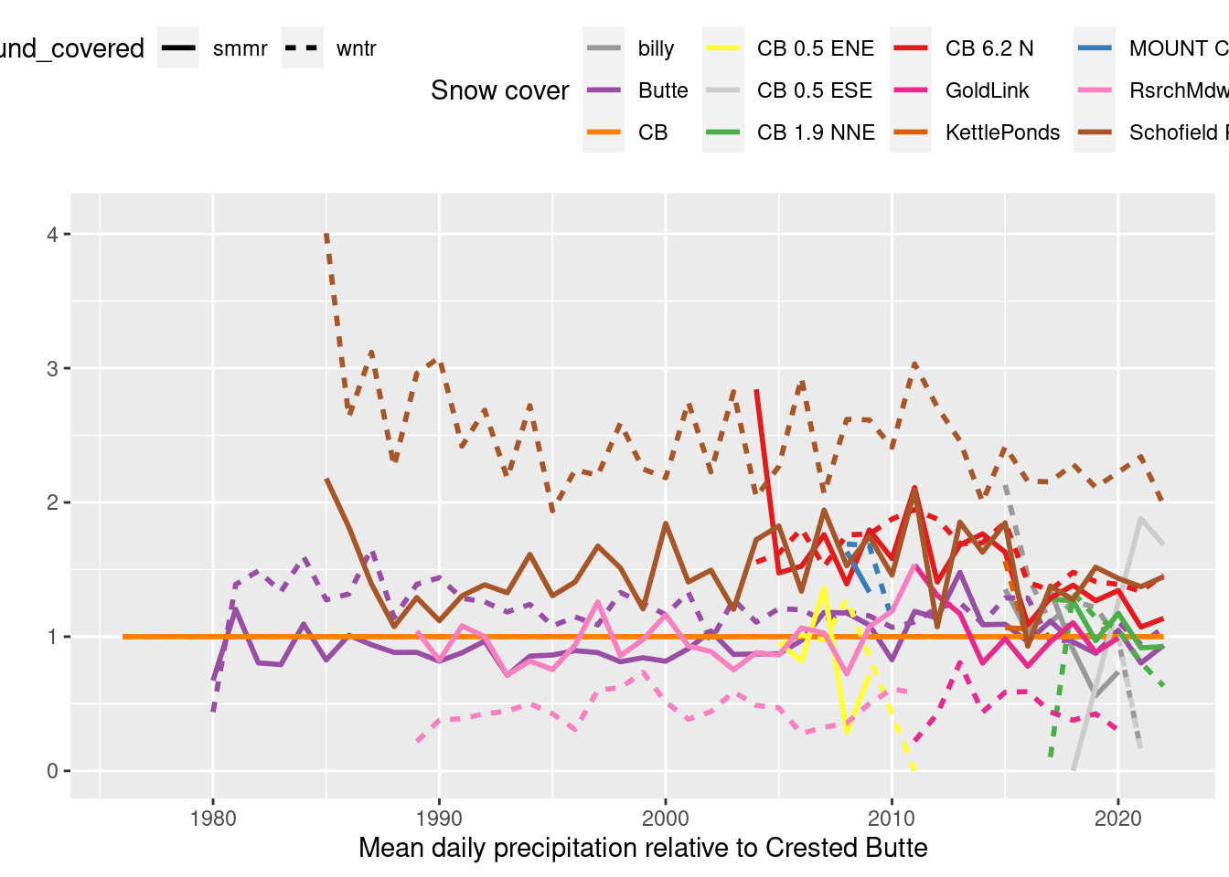
EPA_CB_summer_factor <- relative_to_CB %>% filter(ground_covered=="smmr") %>% drop_na(GTH161) %>% pull(GTH161) %>% mean

daily_filled_7am <- daily_all_7am %>%
  mutate(EPA_NOAA_source = ifelse(is.na(GTH161), ifelse(!is.na(USC00051959), "USC00051959", "missing"), "GTH161"),
         EPA_NOAA_filled = ifelse(is.na(GTH161), ifelse(!is.na(USC00051959), USC00051959*EPA_CB_summer_factor, NA), GTH161))
save(daily_filled_7am, file="data/daily_all.rda")

monthly_filled_7am <- daily_filled_7am %>% group_by(yr = year(date), mo = month(date)) %>%
  summarize(across(-c(date, ground_covered, EPA_NOAA_source),
                   ~ ifelse(sum(is.na(.x))>5, NA, sum(.x, na.rm=T))), .groups="drop") %>%  #tolerate 5 missing days
  arrange(yr, mo)

ggplot(daily_filled_7am %>% mutate(year=year(date)) %>% filter(year>=1989), aes(x=yday(date))) +
  facet_wrap(vars(year)) +
  geom_line(aes(y=40-10*as.integer(ground_covered))) +
  geom_point(aes(y=EPA_NOAA_filled, color=stations_name[EPA_NOAA_source]), size=0.5) +
  scale_color_manual(values=stations_pal)+
  guides(color=guide_legend(override.aes = list(size=3)))+
  labs(x="Day of year", y="EPA/NOAA precipiation (mm)", color="Filled from") +
  theme_minimal() + theme(legend.position="top", panel.spacing = unit(0,"pt"),
                          panel.grid.minor=element_blank(), panel.grid.major.x=element_blank())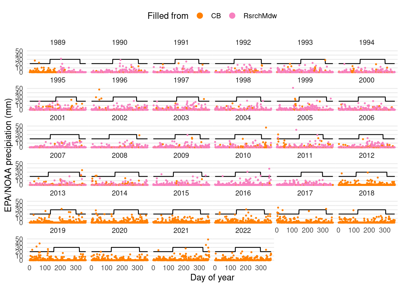
Monthly precip 1989-present
- Recalculated Campbell and Wendlandt 2013 July average, 1989 - 2006 EPA station : 55.8954217 mm
- Maxfield water additions per month: 14 L applied to 4 m2 every 2 days = 1.75 mm daily precip * 31 days in July = 54.25 mm.
monthly_filled_7am %>% filter(yr>=2004) %>%
  pivot_longer(-c(yr,mo), names_to="id", values_to="prcp_mm") %>%
  ggplot(aes(x=mo*30.4-15.2, y=prcp_mm, color=stations_name[id])) + facet_wrap(vars(yr)) + #place points at month midpoint
  #geom_rect(data=waterdates %>% pivot_wider(names_from=precip_treatments, values_from=c(day, date)) %>% mutate(yr=factor(year)),
  #          aes(xmin=day_started, xmax=day_ended, ymin=0, ymax=water_addition_per_month_mm), inherit.aes=F,
  #          fill=water_pal["Addition"])+
  geom_line() +  geom_point()+
    geom_line(data=daily_all_7am  %>% mutate(yr=year(date)) %>% filter(yr>=2004),
              aes(x=yday(date), y=20-20*as.integer(ground_covered)), color="black") +
  labs(y="Monthly precipitation (mm)", x="Day of the year, with snowmelt and first snow dates", color="Station") +
  theme(legend.position="top") + coord_cartesian(ylim=c(0,200)) + scale_color_manual(values=stations_pal)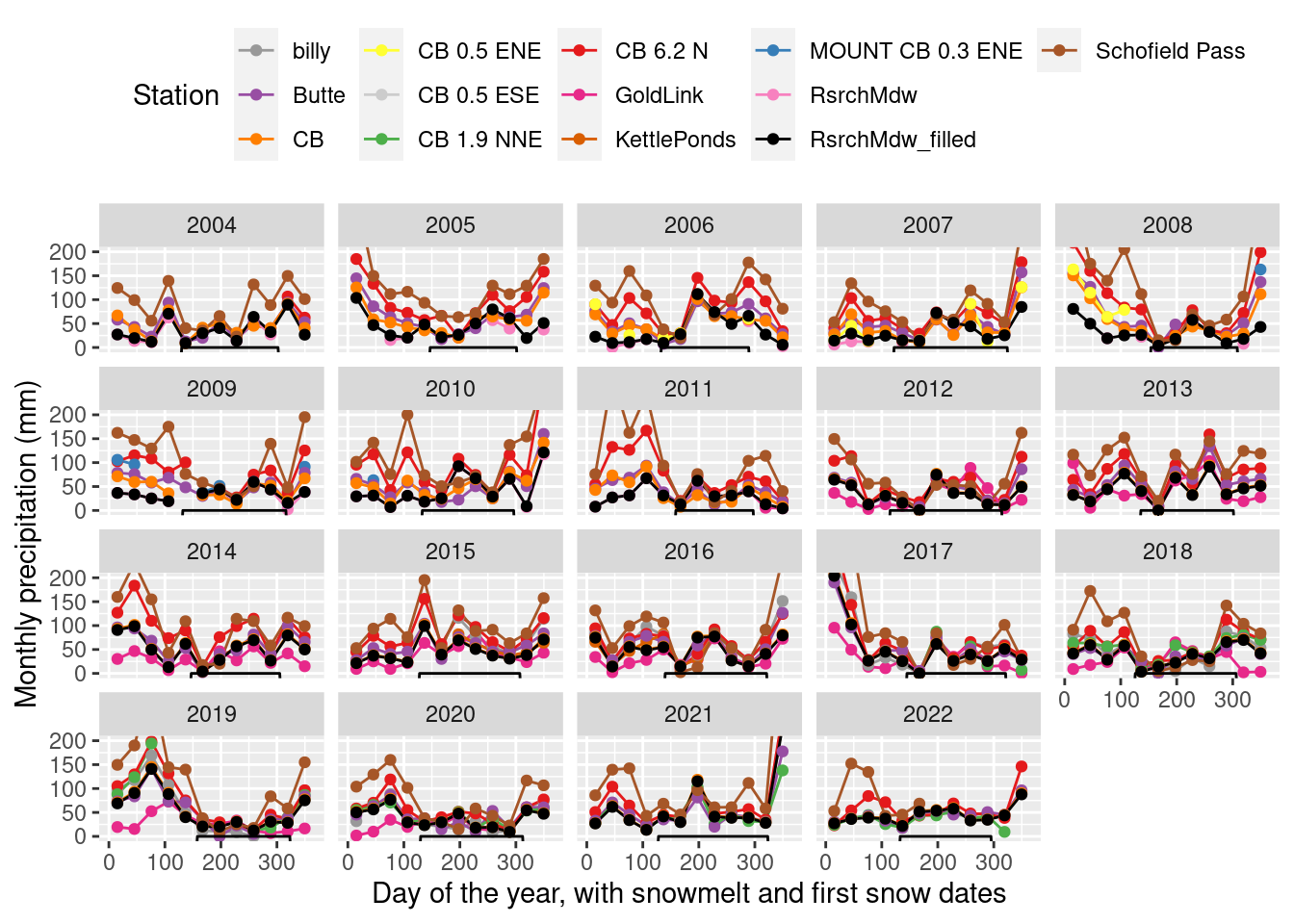
precip_max <- 250
corrplot_monthly_7am <- ggpairs(monthly_all_7am %>% filter(mo %in% 6:9) %>%
          select(-c(yr, mo)) %>% rename_with(~ stations_name[.x]),
        lower=list(continuous=wrap(scatter_continuous), na="blank"),
        upper=list(continuous=wrap(scatter_continuous), na="blank"))
ggsave("images_weather/corrplot_monthly_7am.pdf", corrplot_monthly_7am, device=cairo_pdf, height=10, width=12)

ggplot(monthly_all_7am, aes(y=GTH161,x= USC00051959, color=ifelse(mo %in% 6:9,mo,"Oct - May"))) + geom_point() + geom_smooth(method="lm", se=F) + geom_abline(intercept=0, slope=1) + labs(color="Month")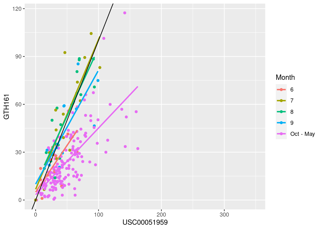
monthly_filled_7am %>% filter(yr >= 1989, mo %in% 5:9) %>%
  ggplot(aes(x=mo,  y=EPA_NOAA_filled)) + geom_smooth(span=0.5, color="black") +
  geom_line(aes(color=ifelse(yr>=2018, "study period (est from CB)", ifelse(yr>=2012,"est from CB","gap-filled EPA data")), group=yr)) +
  geom_point(x=7, y=EPA_89_06_July_avg_mm)+ scale_y_continuous(limits=c(0,100))+
  geom_text(aes(label=ifelse(yr>=2018, yr, "")))  +
  labs(y="Monthly precipitation (mm)", x="Month", title="EPA/NOAA summer precipitation",
       subtitle="Black dot is mean July precipitation 1989-2006", color="Data filling") + theme(legend.position = "top")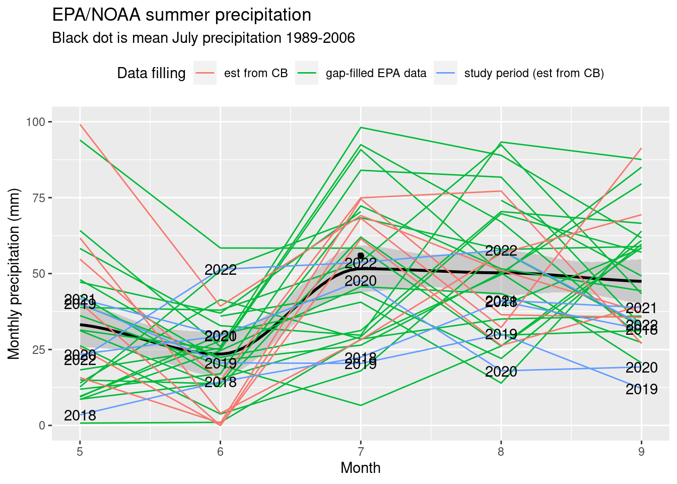
monthly_filled_7am %>% filter(yr >= 1989, mo %in% 5:9) %>% ggplot(aes(x=yr, color=factor(mo), group=mo, shape=ifelse(yr>=2018, "study period (est from CB)", ifelse(yr>=2012,"est from CB","gap-filled EPA data")), y=EPA_NOAA_filled)) +
  geom_vline(xintercept=2011.5) +geom_point() + geom_smooth(se=F, span=0.7) +
  scale_shape_manual(values=c(1,2,19)) + scale_y_continuous(limits=c(0,100))+
  labs(x="Year",y="EPA Research Meadow monthly precipitation (mm)", color="Month", shape="Data filling") +
  geom_segment(data=monthly_filled_7am %>% filter(mo %in% 5:9, yr <= 2007, yr >= 1989,) %>%
                 group_by(mo) %>% summarize(mean_precip=mean(EPA_NOAA_filled)),
aes(x=1989, xend=2006, y=mean_precip, yend=mean_precip, color=factor(mo)), inherit.aes=F, size=1) 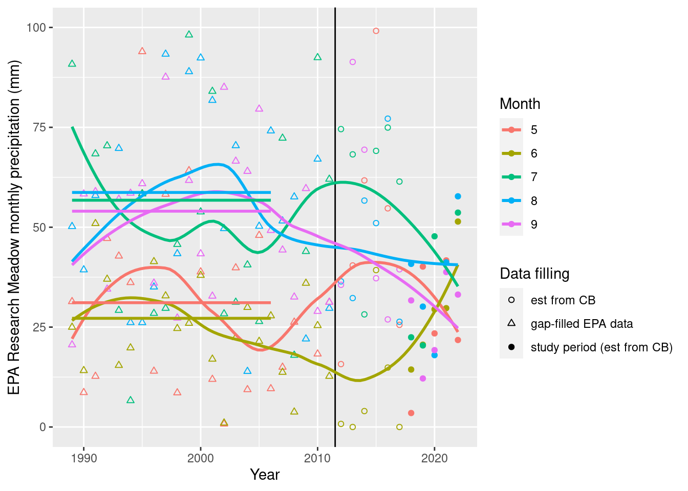
Summer precip trends 1989-present
Combined EPA Research Meadow / NOAA Crested Butte dataset from summers 1990-2020
daily_filled_7am %>% filter(year(date)>1989, year(date)<2023) %>%
  mutate(julian = yday(date), decade = factor(floor(year(date)/10)*10), decade = recode(decade, "2020"="2010")) %>%
  group_by(julian, decade) %>%
  summarize(EPA_NOAA_filled = mean(EPA_NOAA_filled, na.rm=T), ground_covered=mean(as.integer(ground_covered), na.rm=T)-1) %>%
  ggplot(aes(y=EPA_NOAA_filled, x=julian, color=decade)) +
  geom_smooth(span=0.15, se=F)+  geom_point(shape=1, alpha=0.5) +   geom_line(aes(y=ground_covered*2), size=0.75) +
  labs(x="Day of year", y="Mean EPA/NOAA precipiation (mm)", color="Decade", title="Snowmelt and monsoon timing by decade") +
    scale_color_brewer(palette = "Set1", direction = -1) + theme_minimal()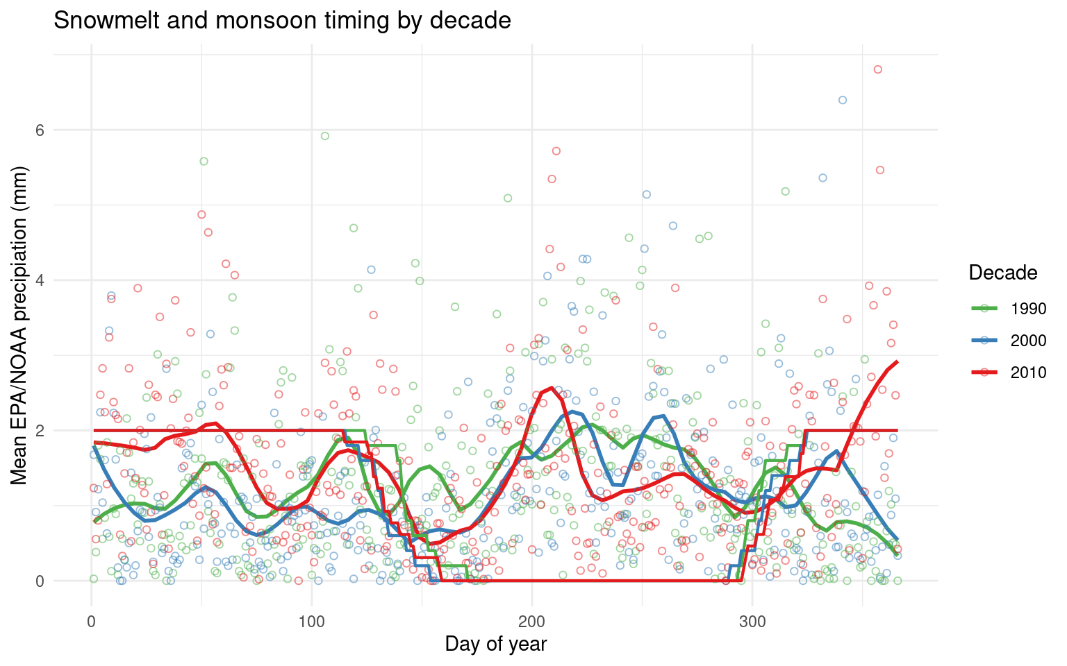
daily_filled_7am %>% filter(year(date)>1989, year(date)<2023, ground_covered=="smmr", EPA_NOAA_filled > 0) %>%
  mutate(decade = factor(floor(year(date)/10)*10), decade = recode(decade, "2020"="2010")) %>% group_by(decade) %>%
  ggplot(aes(x=EPA_NOAA_filled, color=decade)) + geom_density() +
    labs(x="EPA/NOAA precipiation (mm)", y="Proportion", color="Decade", title="Intensity spectrum of summer rainstorms > 0 mm") +
      scale_color_brewer(palette = "Set1", direction = -1) +
  scale_x_continuous(breaks=scales::breaks_extended(10)) + theme_minimal()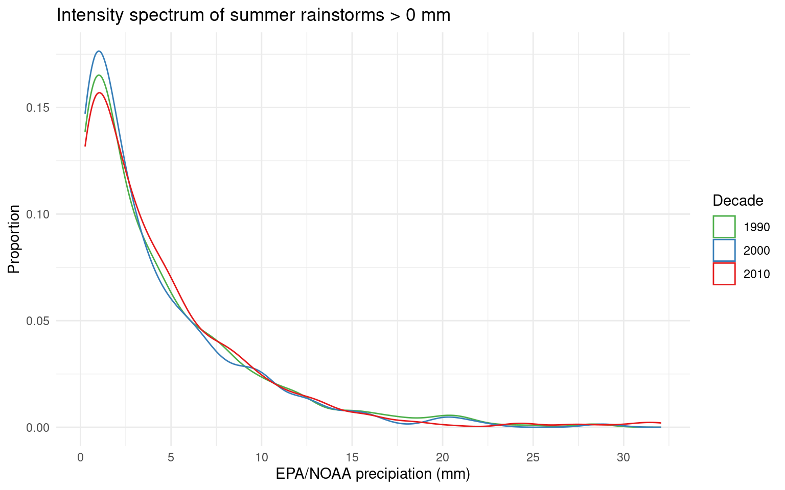
summary_EPA_NOAA <- daily_filled_7am %>% filter(year(date)>1989, year(date)<2023, EPA_NOAA_filled > 2) %>%
  mutate(drought_days = c(0,diff(date)), year=year(date)) %>% filter(ground_covered=="smmr") %>%
  select(year, date, drought_days) %>% group_by(year) %>% summarize(max_drought_days_2mm = max(drought_days)) %>%
  left_join(daily_filled_7am  %>% filter(year(date)>1989, year(date)<2023, ground_covered=="smmr") %>% group_by(year=year(date)) %>%
              summarize(snow_free_days = n(),
                        rain_days_2mm = sum(EPA_NOAA_filled > 2, na.rm=T),
                        prop_rain_days_2mm = rain_days_2mm / snow_free_days,
                        max_precip_mm = max(EPA_NOAA_filled, na.rm=T),
                        avg_precip_mm = mean(EPA_NOAA_filled, na.rm=T),
                        total_precip_mm = sum(EPA_NOAA_filled, na.rm=T),
                        days_until_2mm = min(which(EPA_NOAA_filled> 1)),
                        date_first_2mm = yday(date[days_until_2mm])))

summary_names <- c(snow_free_days = "Snowmelt to first permanent snowfall (d)",
                   max_drought_days_2mm="Longest drought < 2 mm/d (d)",
                   rain_days_2mm = "Days with > 2 mm precip",
                   prop_rain_days_2mm = "Proportion days > 2 mm precip",
                   max_precip_mm = "Maximum precip (mm/d)",
                   avg_precip_mm = "Average precip (mm/d)",
                   total_precip_mm = "Total precip (mm)",
                   days_until_2mm = "Snowmelt to first > 2 mm precip (d)",
                   date_first_2mm = "First > 2 mm precip after snowmelt (day of year)")

summary_EPA_NOAA %>% pivot_longer(!year) %>% filter(name %in% c("avg_precip_mm","max_drought_days_2mm","prop_rain_days_2mm")) %>%
  ggplot(aes(y=value, x=year))+
  facet_wrap(vars(name), scales="free_y", labeller=as_labeller(summary_names)) +
  annotate("rect", xmin=2017.5, xmax=2020.5, ymin=-Inf, ymax=Inf, fill="lightblue")+
  geom_smooth(method="lm", color="black", se=F) + geom_point(color="grey60") + labs(x="Year", y="") +
  scale_y_continuous(limits=c(0, NA), expand = expansion(mult=c(0, 0.05))) +
  #stat_poly_eq(formula = y ~ x, aes(label = paste(..eq.label.., ..rr.label.., ..p.value.label.., sep = "~~~")), parse = T) +
  theme_minimal() +theme(axis.title.y= element_blank(), text=element_text(color="black", size=14),
                         axis.text = element_text(color="black"),  panel.border = element_rect(fill=NA, colour = "black"))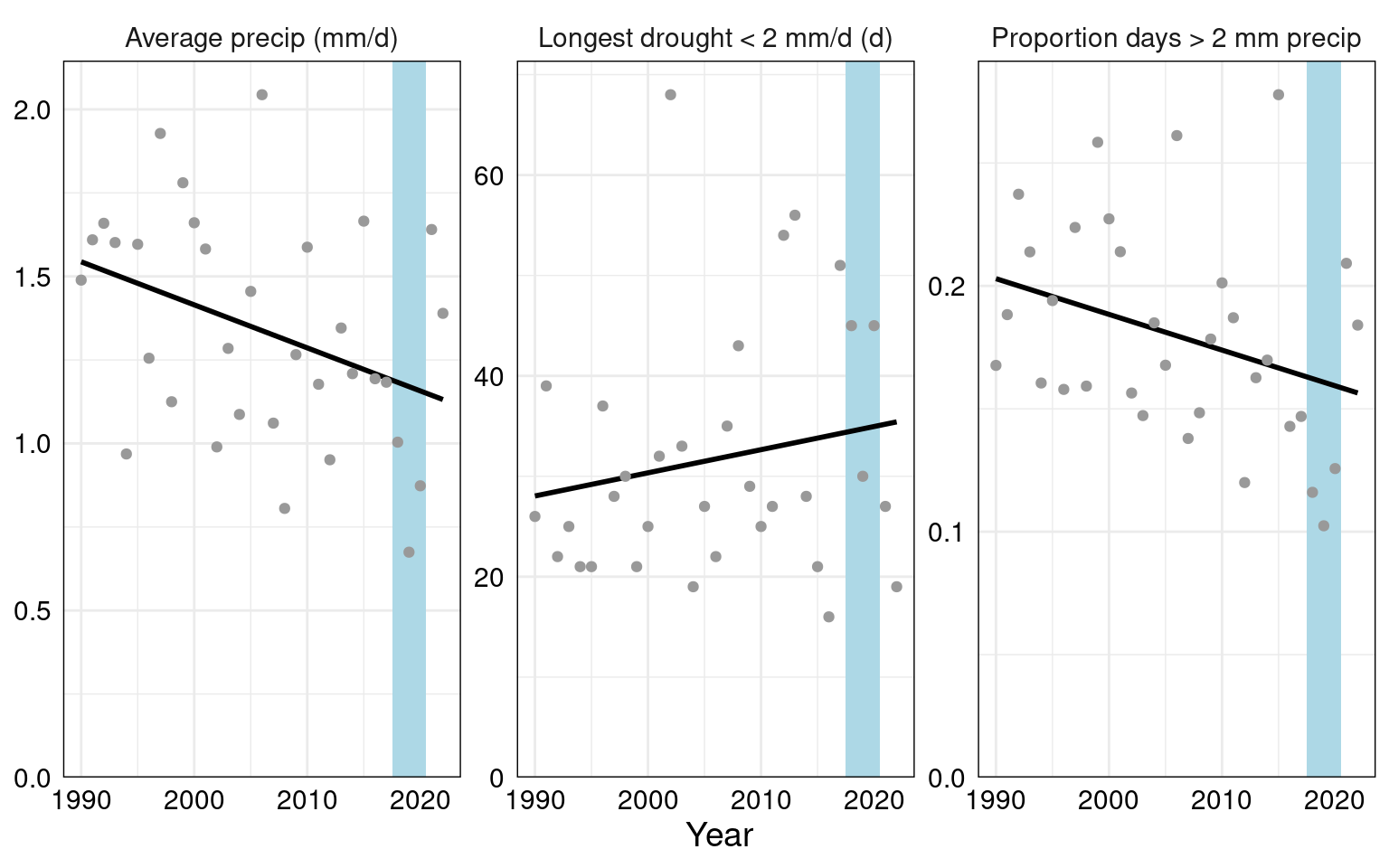
summary_EPA_NOAA %>% summarize(across(-year, mean, na.rm=T)) %>% kable(caption = "Averages 1990-2020")| max_drought_days_2mm | snow_free_days | rain_days_2mm | prop_rain_days_2mm | max_precip_mm | avg_precip_mm | total_precip_mm | days_until_2mm | date_first_2mm |
|---|---|---|---|---|---|---|---|---|
| 31.72727 | 168.8485 | 30.24242 | 0.1796958 | 21.88878 | 1.337604 | 224.0971 | 6.515151 | 144.2121 |
summary_EPA_NOAA %>% summarize(across(-year, sd, na.rm=T)) %>% kable(caption = "Standard deviation 1990-2020")| max_drought_days_2mm | snow_free_days | rain_days_2mm | prop_rain_days_2mm | max_precip_mm | avg_precip_mm | total_precip_mm | days_until_2mm | date_first_2mm |
|---|---|---|---|---|---|---|---|---|
| 12.30161 | 16.57581 | 7.685336 | 0.0430214 | 6.017044 | 0.3337806 | 55.83056 | 7.980919 | 15.33125 |
library(broom)
summary_EPA_NOAA %>% pivot_longer(!year) %>% group_by(name) %>% nest() %>%
  mutate(model = map(data, ~ lm(value ~ year, data = .)),
coefs = map(model, tidy)) %>% select(-c(data, model)) %>% unnest(coefs) %>% kable(caption = "Regression coefficients 1990-2020")| name | term | estimate | std.error | statistic | p.value |
|---|---|---|---|---|---|
| max_drought_days_2mm | (Intercept) | -430.8863636 | 450.7708097 | -0.9558879 | 0.3465243 |
| max_drought_days_2mm | year | 0.2306150 | 0.2247087 | 1.0262840 | 0.3126997 |
| snow_free_days | (Intercept) | -1124.4583333 | 572.2776455 | -1.9648825 | 0.0584445 |
| snow_free_days | year | 0.6447193 | 0.2852798 | 2.2599544 | 0.0309964 |
| rain_days_2mm | (Intercept) | 301.7765152 | 282.1763060 | 1.0694609 | 0.2931190 |
| rain_days_2mm | year | -0.1353610 | 0.1406646 | -0.9622961 | 0.3433475 |
| prop_rain_days_2mm | (Intercept) | 3.0937835 | 1.5151474 | 2.0419026 | 0.0497483 |
| prop_rain_days_2mm | year | -0.0014527 | 0.0007553 | -1.9233248 | 0.0636658 |
| max_precip_mm | (Intercept) | 71.0029630 | 224.0247108 | 0.3169425 | 0.7534119 |
| max_precip_mm | year | -0.0244836 | 0.1116761 | -0.2192380 | 0.8279018 |
| avg_precip_mm | (Intercept) | 27.1836715 | 11.5380077 | 2.3560109 | 0.0249749 |
| avg_precip_mm | year | -0.0128844 | 0.0057517 | -2.2401059 | 0.0323930 |
| total_precip_mm | (Intercept) | 2870.5208184 | 2025.2469564 | 1.4173683 | 0.1663484 |
| total_precip_mm | year | -1.3192541 | 1.0095833 | -1.3067313 | 0.2009154 |
| days_until_2mm | (Intercept) | -108.1325758 | 296.6595995 | -0.3645005 | 0.7179590 |
| days_until_2mm | year | 0.0571524 | 0.1478845 | 0.3864666 | 0.7017912 |
| date_first_2mm | (Intercept) | 617.5530303 | 564.8892643 | 1.0932285 | 0.2827163 |
| date_first_2mm | year | -0.2359626 | 0.2815967 | -0.8379452 | 0.4084759 |
Summer precip trends 1909-present
All data from NOAA Crested Butte station.
#weird long run of high precipitation in Sept 1927
daily_NOAA %>% filter(id=="USC00051959", year(date)>1909, year(date)!=1927) %>%
  mutate(julian = yday(date), decade = factor(floor(year(date)/10)*10), decade = recode(decade, "2020"="2010")) %>%
  group_by(julian, decade) %>% summarize(prcp_mm = mean(prcp_mm, na.rm=T)) %>%
  ggplot(aes(y=prcp_mm, x=julian, color=decade)) + geom_smooth(span=0.15, se=F)+
  labs(x="Day of year", y="Mean Crested Butte precipiation (mm)", color="Decade", title="Snowmelt and monsoon timing by decade") +
  scale_color_viridis_d(option="inferno") + coord_cartesian(xlim=c(120,270)) + theme_dark()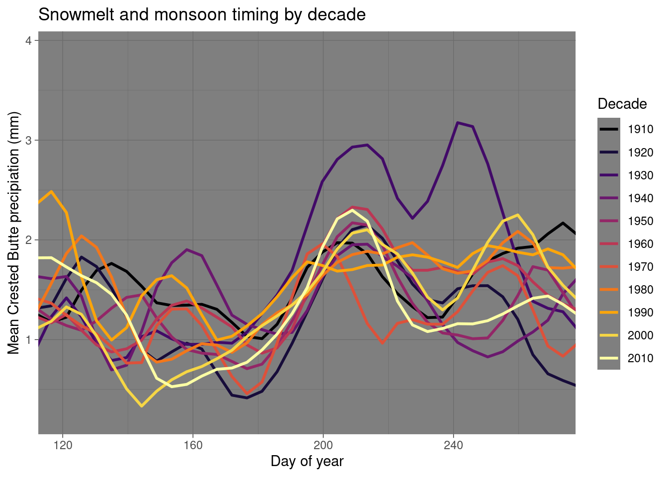
daily_NOAA %>% filter(id=="USC00051959", year(date)>1909, year(date)!=1927,yday(date)>=120, yday(date)<= 270, prcp_mm > 0) %>%
  mutate(decade = factor(floor(year(date)/10)*10), decade = recode(decade, "2020"="2010")) %>% group_by(decade) %>%
  ggplot(aes(x=prcp_mm, color=decade)) + geom_density() +
    labs(x="Crested Butte precipiation (mm)", y="Proportion", color="Decade",
         title="Intensity spectrum of rainstorms > 0 mm \n(day 120-270, Crested Butte)") +
    scale_color_viridis_d(option="inferno") +  coord_cartesian(xlim=c(0,40)) +  theme_dark()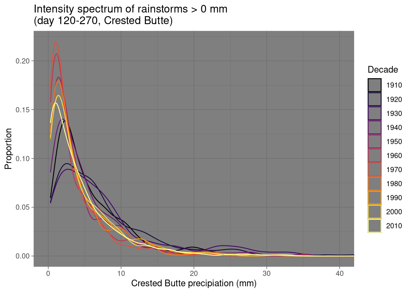
daily_NOAA %>% filter(id=="USC00051959", year(date)>1909, year(date)!=1927,prcp_mm > 2) %>%
  mutate(drought_days = c(0,diff(date)), year=year(date)) %>% filter(yday(date)>=120, yday(date)<= 270,) %>%
  select(year, date, drought_days) %>% group_by(year) %>% summarize(max_drought_days = max(drought_days)) %>%
  ggplot(aes(x= year, y=max_drought_days)) + geom_smooth(span=0.5) +geom_point() +
  labs(x="Year", y="Consecutive drought days with < 2 mm daily precipitation \n(day 120-270, Crested Butte)")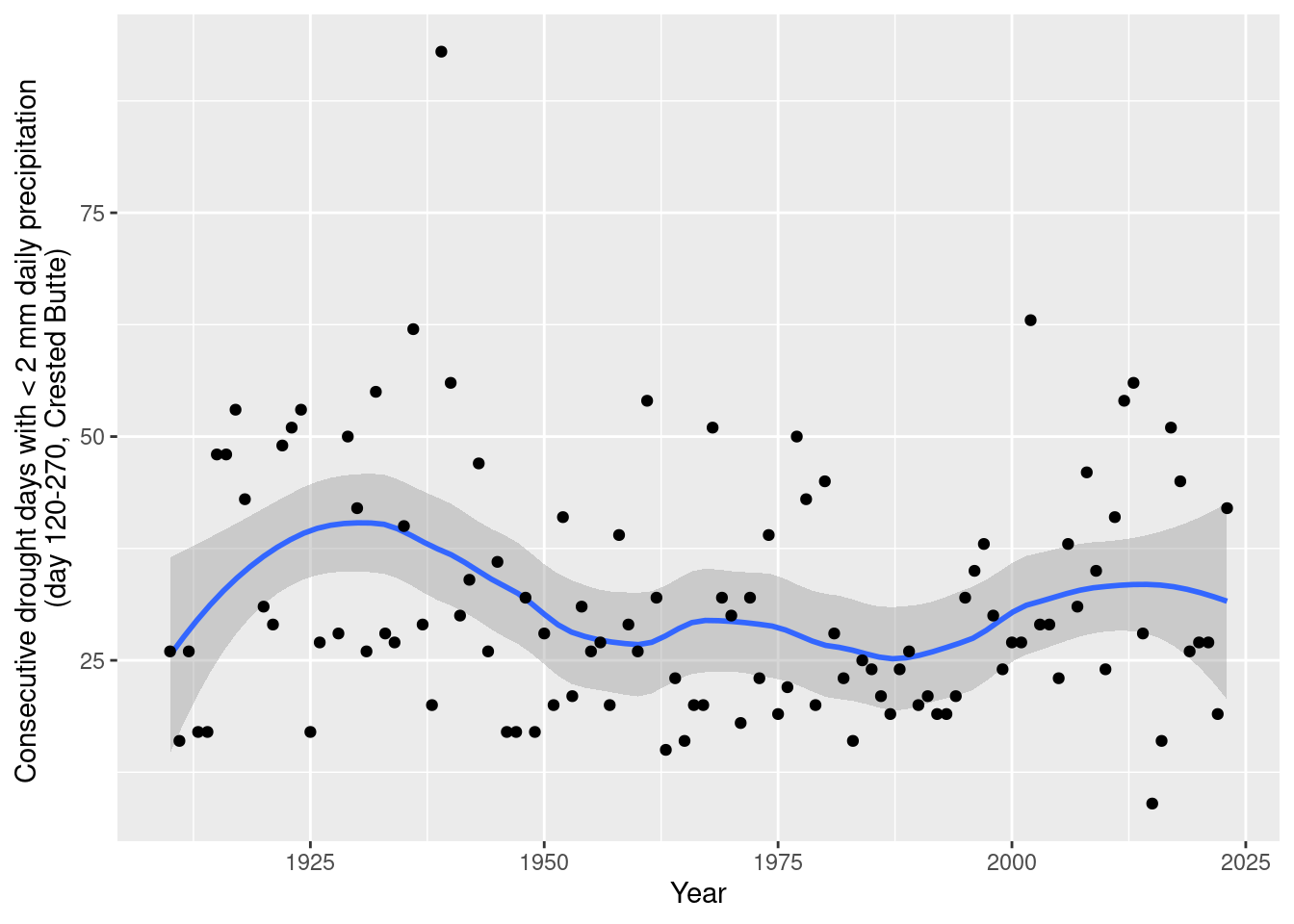
daily_NOAA %>% filter(id=="USC00051959", year(date)>1909, year(date)!=1927,yday(date)>=120, yday(date)<= 270, prcp_mm > 2) %>%
  count(year=year(date)) %>%
    ggplot(aes(x= year, y=n)) + geom_smooth(span=0.5) + geom_point() +
  labs(x="Year", y="Days with > 2 mm daily precipitation (day 120-270, Crested Butte)")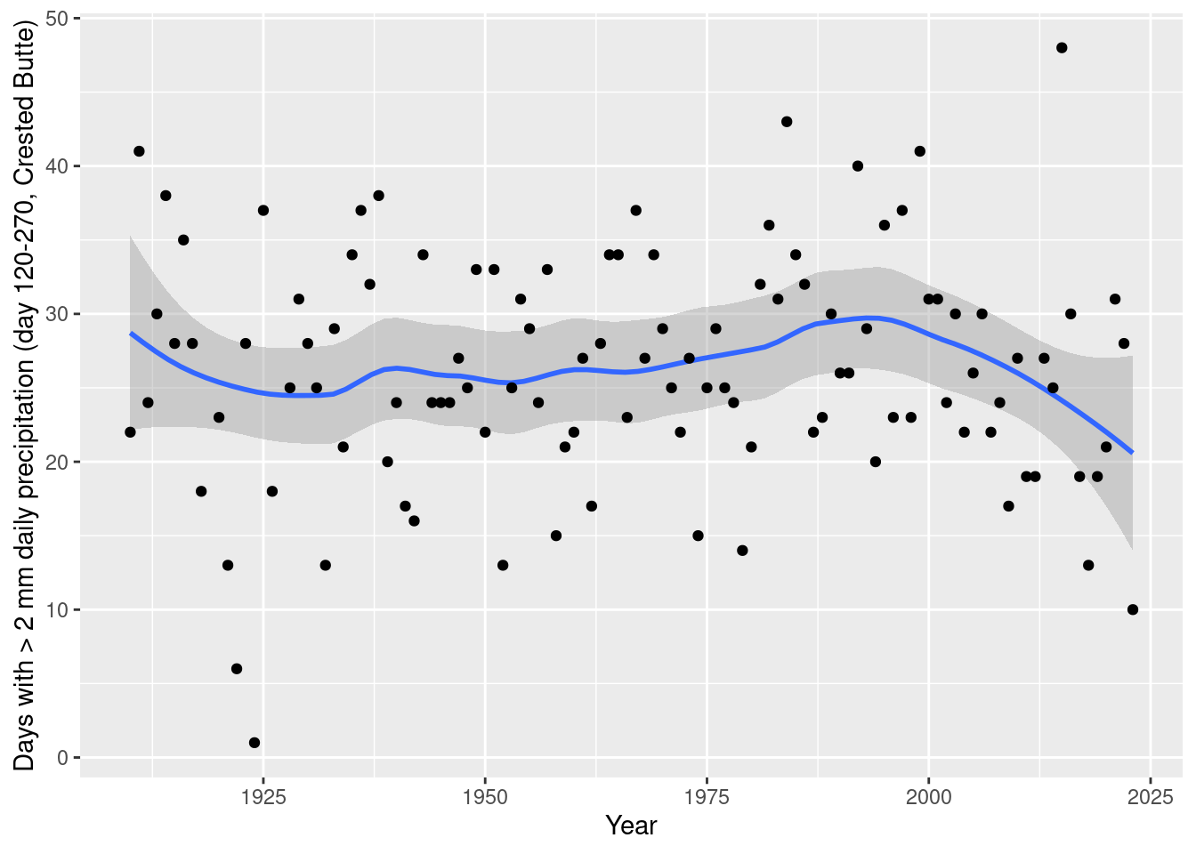
daily_NOAA %>% filter(id=="USC00051959", year(date)>1909, year(date)!=1927, yday(date)>=120, yday(date)<= 270) %>%
  group_by(year=year(date)) %>% summarize(total_mm=sum(prcp_mm, na.rm=T)) %>%
    ggplot(aes(x= year, y=total_mm)) + geom_smooth(span=0.5) + geom_point() +
  labs(x="Year", y="Total precipitation (mm, day 120-270, Crested Butte)")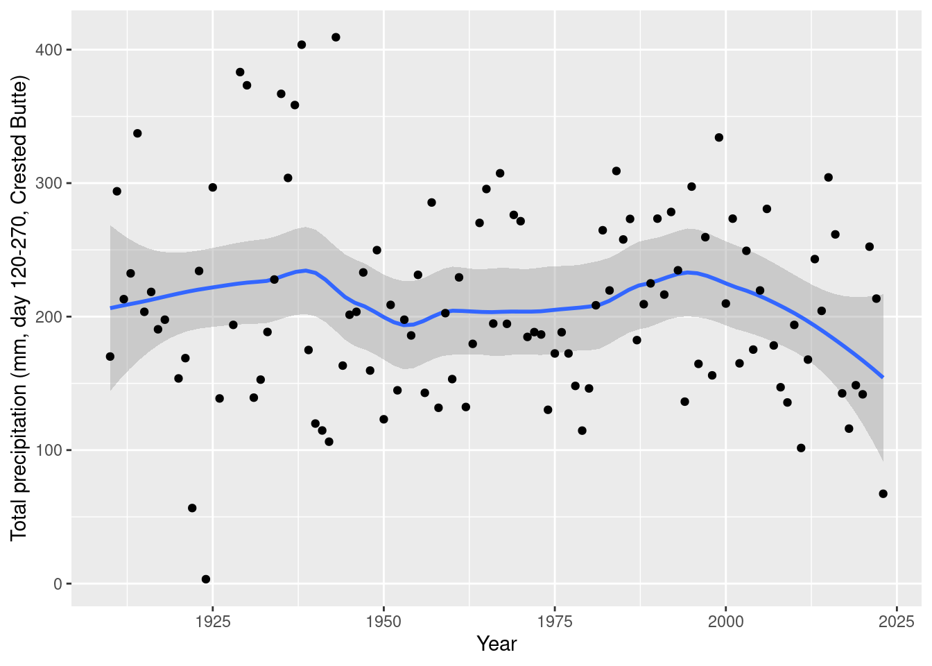
daily_NOAA %>% filter(id=="USC00051959", year(date)>1909, yday(date)>=120, yday(date)<= 270) %>%
  group_by(year=year(date)) %>% summarize(tmax_mean=mean(tmax_C, na.rm=T)) %>%
    ggplot(aes(x= year, y=tmax_mean)) + geom_smooth(span=0.3) + geom_point() +
  labs(x="Year", y="Average maximum temperature (C, day 120-270, Crested Butte)")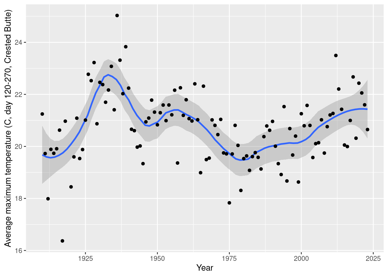
daily_NOAA %>% filter(id=="USC00051959", year(date)>1909, yday(date)>=120, yday(date)<= 270) %>%
  group_by(year=year(date)) %>% summarize(tmin_mean=mean(tmin_C, na.rm=T)) %>%
    ggplot(aes(x= year, y=tmin_mean)) + geom_smooth(span=0.3) + geom_point() +
  labs(x="Year", y="Average minimum temperature (C, day 120-270, Crested Butte)")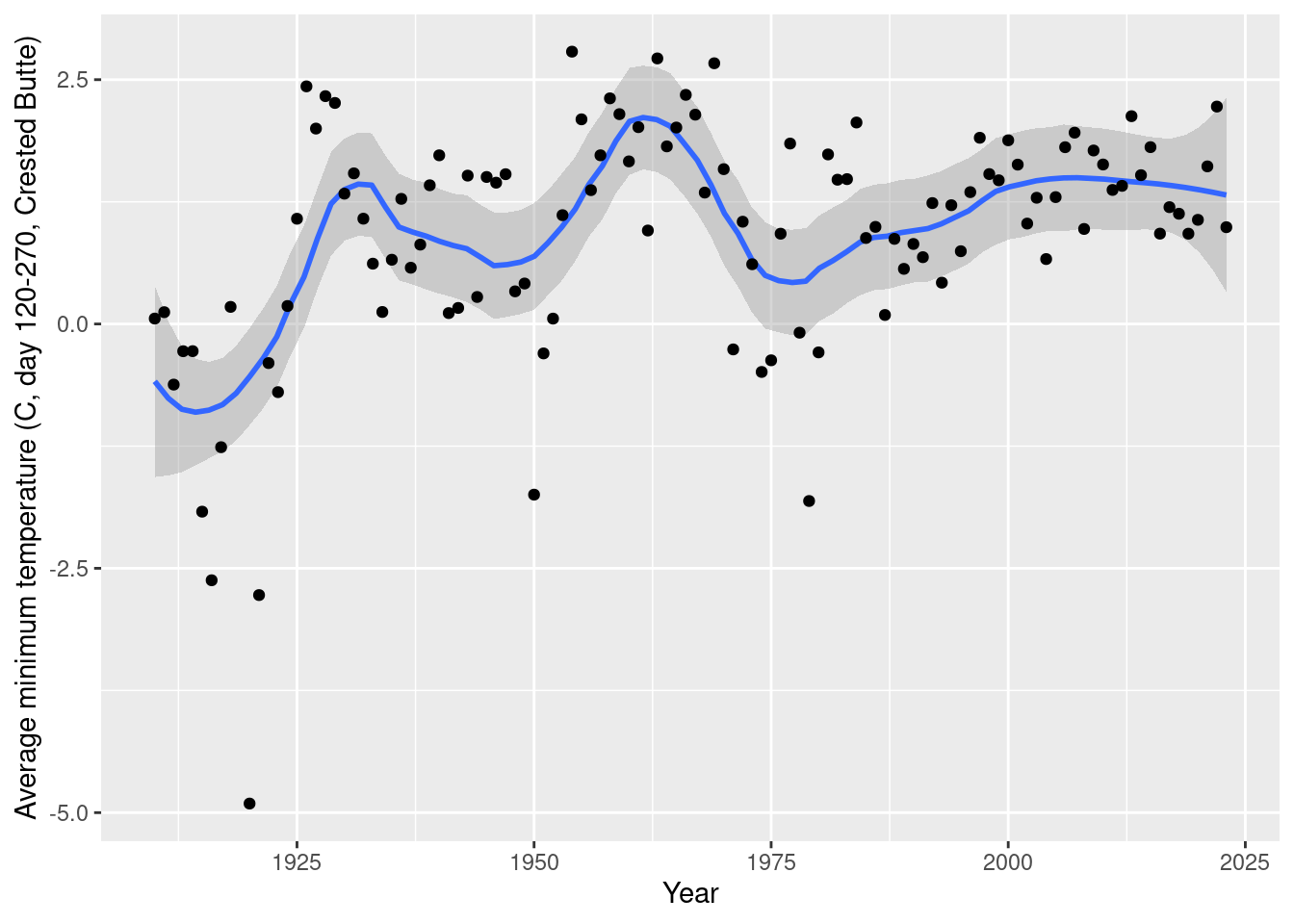
Summer temperature trends 1909-present
ggplot(daily_GTH161, aes(y=TEMPERATURE, x= date, color=month(date) %in% 5:7))+ geom_line(aes(group=1)) + labs(color="May-July", title="GTH161 mean temp")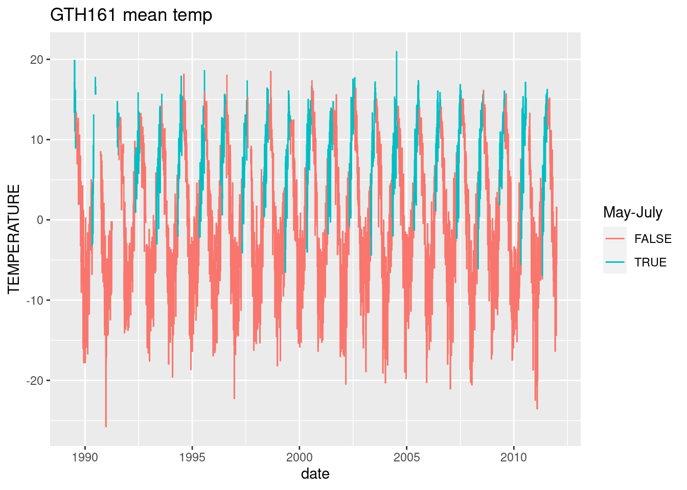
daily_GTH161 %>% filter(month(date) %in% 5:7) %>% group_by(year=year(date)) %>% summarize(days_missing=sum(is.na(TEMPERATURE))) %>% print(n=23)#too much missing temp data# A tibble: 23 × 2
year days_missing
<dbl> <int>
1 1989 0
2 1990 58
3 1991 61
4 1992 9
5 1993 0
6 1994 2
7 1995 6
8 1996 0
9 1997 8
10 1998 17
11 1999 0
12 2000 19
13 2001 14
14 2002 0
15 2003 0
16 2004 16
17 2005 0
18 2006 9
19 2007 0
20 2008 0
21 2009 0
22 2010 0
23 2011 0ggplot(daily_NOAA %>% filter(id=="USC00051959"), aes(y=tmax_C, x= date))+ geom_line() + labs("CB max temp") #CB station does not have mean temp, only max and min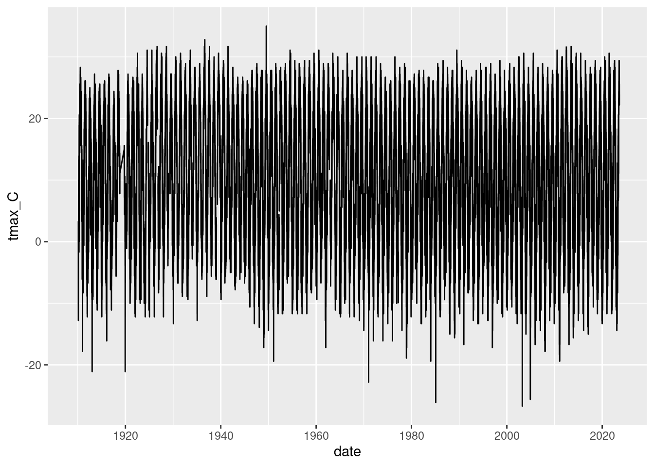
daily_NOAA  %>% filter(id=="USC00051959", year(date)>1909, month(date) %in% 5:7) %>% group_by(year=year(date)) %>%
  summarize(tmax_C_mean = mean(tmax_C, na.rm=T), days_missing=sum(is.na(tmax_C))) %>% ggplot(aes(x=year, y=tmax_C_mean)) + geom_point() + geom_smooth()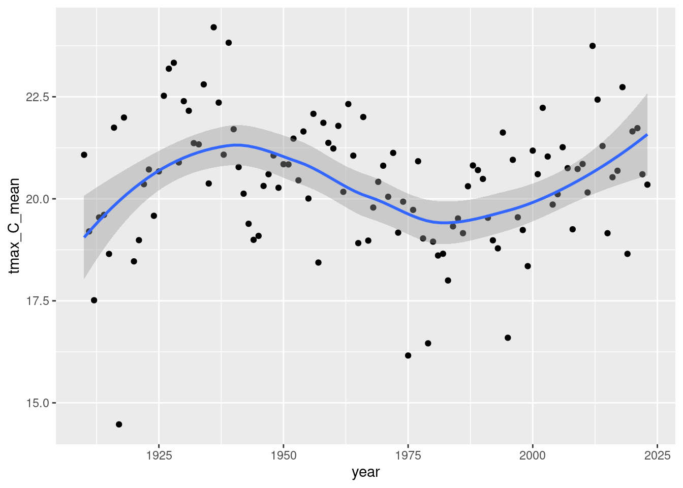
Snowmelt timing 1976-present
groundcover %>% mutate(first_snow_day=first_snow_day-365) %>%
  pivot_longer(ends_with("day"), names_to="threshold", values_to="day") %>% drop_na(day) %>% select(-starts_with("first")) %>%
  mutate(threshold = fct_reorder(factor(threshold),day, na.rm=T, .desc=T)) %>%
  ggplot(aes(x=year, y=day, color=threshold)) +
  geom_line(aes(group=year), size=2)+ geom_smooth( method="lm", se=F) +geom_point() +
  scale_x_continuous(minor_breaks = 1976:2022, position = "top") + scale_y_continuous(n.breaks=10)+
  scale_color_grey(labels=function(x) str_to_sentence(str_replace_all(x, "_", " ")), start=0, end=0.85) +
  labs(x="Year", y="Day of year", color="Threshold") + theme_minimal()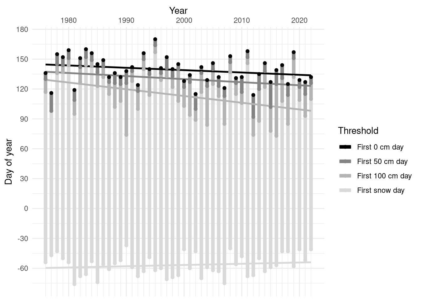
list("0cm"=coef(lm(first_0_cm_day ~ year, data=groundcover)),
     "50cm"=coef(lm(first_50_cm_day ~ year, data=groundcover)),
     "100cm"=coef(lm(first_100_cm_day ~ year, data=groundcover)),
     "firstsnow"=coef(lm(first_snow_day ~ year, data=groundcover))) %>%
bind_rows(.id="first_day_at") %>% select(-`(Intercept)`) %>% kable(caption="Change per year, 1980-2022", digits=2)| first_day_at | year |
|---|---|
| 0cm | -0.24 |
| 50cm | -0.31 |
| 100cm | -0.68 |
| firstsnow | 0.12 |